在生產環境中將 GraphRAG 的 Token 成本砍掉 90%

文章資訊

作者：Alexander Shereshevsky　　日期：2026-06-13

原文標題：Cutting GraphRAG Token Costs by 90% in Production

Medium 原連結：https://medium.com/graph-praxis/cutting-graphrag-token-costs-by-90-in-production-5885b3ffaef0

⭐ 收藏

🎧 摘要語音

🔊 朗讀全文（收藏後自動生成）

---

📝 重點摘要

TL;DR

透過 schema 約束抽取與分層檢索路由，GraphRAG 成本降九成且準確率反升。

核心問題

標準 GraphRAG（如微軟原版）在「圖譜建構」與「查詢檢索」兩階段大量呼叫 LLM，導致中型語料庫索引成本動輒數萬美元。本文拆解作者在生產系統中將成本壓到約十分之一、同時提升準確率的具體技術決策。

關鍵發現 / 數據

• 每千份文件索引 token 從 ~2.5M 降至 ~230K（−90.7%），月 API 成本從 $14,200 降至 $1,680（−88%）。
• Schema 約束抽取使每段三元組從 15–30 個降至 3–8 個高品質三元組，輸出 token 減 70–80%。
• 多跳準確率不降反升：HotpotQA +8.4%、2Wiki +60.7%（48.3% → 77.6%）。
• 約 40% 查詢在 L₁/L₂ 層解決，不觸及昂貴的社群摘要層；另約 25% 直接回退到向量 RAG。
• 對比方法：TERAG 以 3–11% token 達 80%+ 準確率；LinearRAG 零 LLM 索引在 2WikiMultiHopQA 達 70.20 Contain-Acc。

方法亮點

• Schema-guided 抽取：限定實體/關係/屬性類型，輸出空間受限，並以信心分數自動擴充 schema。
• 雙感知社群偵測：結合拓撲（Jaccard）與語義（embedding cosine）相似度（α=0.6），改善 Leiden 在知識圖上的不穩定。
• 四層知識樹（L₁–L₄）：依查詢類型路由到不同粒度，只為所需粒度付費。
• Agentic 查詢分解 + 反思迴圈：將多跳查詢拆成平行子查詢並評估完整性，避免過度/不足檢索。

對我的研究有用嗎？

非常值得參考。「schema 約束抽取降噪反而提升下游準確率」對 LLM Graph 建構是核心洞見；雙感知社群偵測補足純拓撲 Leiden 的缺陷，可用於 community-based GraphRAG。最有方法論價值的是 AnonyRAG 匿名化評估——用不透明 ID 替換實體，分離「檢索貢獻」與「參數知識」，這對誠實評估 GraphRAG 檢索品質極具參考性。文末對 KET-RAG、TERAG、LinearRAG、HippoRAG2 等的橫向比較也是不錯的 survey 入口。

評語

值得一讀的實務導向好文，附程式碼與引用；但成本/準確率數字來自作者自家系統、缺乏可複現細節，宜當作工程啟發而非嚴謹 benchmark。

---

🌐 中英對照

Author: Alexander Shereshevsky Published: Source: https://medium.com/graph-praxis/cutting-graphrag-token-costs-by-90-in-production-5885b3ffaef0 Fetched: 2026-06-13T00:38:23.699205

---

Cutting GraphRAG Token Costs by 90% in Production / 在生產環境中將 GraphRAG 的 Token 成本削減 90%

Press enter or click to view image in full size

按下 Enter 鍵或點擊以檢視全尺寸圖片

A practical guide to the architecture decisions, algorithms, and implementation tricks that make graph-based RAG affordable at scale.

一份實用指南，介紹那些讓「基於圖的檢索增強生成 (Graph-based RAG)」能在大規模場景下負擔得起的架構決策、演算法與實作技巧。

If you’ve built a RAG system that goes beyond simple vector retrieval — one that synthesizes answers across documents, handles multi-hop reasoning, or navigates complex domain knowledge — you’ve probably looked at GraphRAG. And if you’ve looked at GraphRAG, you’ve probably looked at the bill and put it back on the shelf.

如果你曾建立過超越簡單向量檢索 (Vector Retrieval) 的 RAG 系統——一個能跨文件綜合出答案、處理多跳推理 (Multi-hop Reasoning)，或在複雜領域知識中導航的系統——你大概看過 GraphRAG。而如果你看過 GraphRAG，你大概也看了一眼帳單，然後就把它束之高閣了。

We didn’t. We’re running a vertically unified agentic GraphRAG architecture in production, and it costs us roughly one-tenth of what a naive graph-based RAG would. This article breaks down the specific technical decisions that got us there, maps them against the broader research landscape over the past six to eight months, and includes enough implementation detail for you to start applying these ideas to your own pipelines.

我們沒有。我們在生產環境中運行著一套垂直統一的代理式 (Agentic) GraphRAG 架構，其成本大約只有樸素 (Naive) 基於圖的 RAG 的十分之一。本文拆解了讓我們達成這一點的具體技術決策，將它們對照過去六到八個月更廣泛的研究全貌，並包含足夠的實作細節，讓你能開始將這些想法應用到自己的管線 (Pipeline) 中。

The Cost Anatomy of Standard GraphRAG / 標準 GraphRAG 的成本剖析

Before optimizing, you need to understand where tokens are actually being spent. A standard GraphRAG pipeline has two major cost centers: graph construction (indexing) and graph retrieval (query-time).

在進行優化之前，你需要了解 token 究竟花在哪裡。一個標準的 GraphRAG 管線有兩大成本中心：圖構建 (Graph Construction，即索引建立) 與圖檢索 (Graph Retrieval，即查詢時)。

Graph construction in Microsoft’s original GraphRAG approach works like this: every document chunk gets sent to an LLM with a prompt like “Extract all entities and relationships from the following text.” The LLM returns entity-relation triplets, which are assembled into a knowledge graph. Then the graph is partitioned into communities using the Leiden algorithm, and each community gets summarized by — you guessed it — another LLM call. For hierarchical community detection, this repeats at multiple levels.

圖構建 在微軟原始的 GraphRAG 方法中是這樣運作的：每個文件分塊 (Chunk) 都會被送進一個大型語言模型 (LLM)，搭配類似 「從以下文本中提取所有實體與關係」 的提示詞 (Prompt)。LLM 回傳實體—關係三元組 (Entity-relation Triplet)，這些三元組被組裝成一個知識圖譜 (Knowledge Graph)。接著，使用 Leiden 演算法將圖劃分成社群 (Community)，而每個社群都由——你猜對了——另一次 LLM 呼叫來進行摘要。對於階層式社群偵測 (Hierarchical Community Detection)，這個過程會在多個層級上重複進行。

For a corpus of 10,000 documents at ~500 tokens per chunk, with 3–5 extraction calls per chunk and community summarization across 3–4 levels, you’re looking at 50,000–200,000 LLM calls just for indexing. At current API pricing, that can easily reach tens of thousands of dollars for a moderately sized corpus.

對於一個包含 10,000 份文件、每個分塊約 500 個 token 的語料庫 (Corpus)，每個分塊有 3 到 5 次提取呼叫，加上跨 3 到 4 個層級的社群摘要，光是建立索引你就要面對 50,000 到 200,000 次的 LLM 呼叫。以目前的 API 定價，對於一個中等規模的語料庫，這很容易就達到數萬美元。

Graph retrieval adds to the tab. Global search fans out, map-reduce-style, across community summaries. Local search traverses entity neighborhoods and stuffs context windows with relationship descriptions. DRIFT search improved things by combining global and local approaches, but it still requires significant LLM processing at query time.

圖檢索 則進一步增加了帳單。全域搜尋 (Global Search) 以 map-reduce 的方式在社群摘要間扇出展開 (Fan out)。局部搜尋 (Local Search) 遍歷實體鄰域，並用關係描述塞滿上下文視窗 (Context Window)。DRIFT 搜尋透過結合全域與局部方法改善了情況，但它在查詢時仍需要大量的 LLM 處理。

Pipeline Stage                             Typical Token Consumption Range (% of Total)    
 ------------------------------------------ ----------------------------------------------   
  (1) Entity/Relation Extraction             45% – 55%                                       
  (2) Community Summarization                25% – 35%                                       
  (3) Query-time Map-Reduce over Summaries   10% – 15%                                       
  (4) Answer Generation                      5% – 10%

Token Cost Breakdown of a Standard GraphRAG Pipeline

標準 GraphRAG 管線的 Token 成本分解

Optimization 1: Schema-Guided Extraction / 優化一：綱要引導式提取 (Schema-Guided Extraction)

The single highest-leverage optimization is constraining what you extract. Open-ended extraction (“find all entities and relationships”) is expensive and noisy. Schema-guided extraction gives the LLM a bounded target.

槓桿效益最高的單一優化，就是限制你所提取的內容。開放式提取 (Open-ended Extraction，即「找出所有實體與關係」) 既昂貴又充滿雜訊。綱要引導式提取則給予 LLM 一個有界的目標。

The approach defines a seed schema as a triplet:

該方法將一個種子綱要 (Seed Schema) 定義為一個三元組：

Schema = ⟨ Sₑ, Sᵣ, Sₐₜₜᵣ ⟩

Where Sₑ is the set of entity types, Sᵣ is the set of relation types, and Sₐₜₜᵣ is the set of attribute types. The extraction agent performs constrained generation — its output space is limited to the Cartesian product Sₑ × Sᵣ × Sₑ, plus attribute assignments from Sₐₜₜᵣ.

其中 Sₑ 是實體類型 (Entity Type) 的集合，Sᵣ 是關係類型 (Relation Type) 的集合，而 Sₐₜₜᵣ 是屬性類型 (Attribute Type) 的集合。提取代理 (Extraction Agent) 執行受約束的生成 (Constrained Generation)——其輸出空間被限制在笛卡兒積 (Cartesian Product) Sₑ × Sᵣ × Sₑ，外加來自 Sₐₜₜᵣ 的屬性指派。

Here’s what this looks like in practice. Instead of this prompt:

實際操作起來是這個樣子。與其使用這個提示詞：

Extract all entities and relationships from the following text.  
Return them as JSON triplets.

You send this:

你改送出這個：

Given the following schema:  
  Entity types: [Person, Organization, Drug, Disease, Gene]  
  Relation types: [treats, causes, works_at, regulates, interacts_with]  
  Attribute types: [dosage, mechanism, severity, role]  

Extract entity-relation-attribute triplets that conform to this schema.  
Return ONLY triplets matching the defined types. Ignore all other entities.

The difference in output token count is dramatic. Open-ended extraction on a biomedical paragraph might return 15–30 triplets, many of which are noise (dates, locations, generic concepts). Schema-guided extraction on the same paragraph returns 3–8 high-quality triplets. That’s a 70–80% reduction in the number of output tokens per chunk, and the extracted graph is cleaner.

輸出 token 數量的差異是巨大的。對一段生物醫學段落進行開放式提取，可能會回傳 15 到 30 個三元組，其中許多是雜訊（日期、地點、泛用概念）。對同一段落進行綱要引導式提取則回傳 3 到 8 個高品質的三元組。這是每個分塊輸出 token 數量 70% 到 80% 的削減，而且提取出的圖也更乾淨。

The schema isn’t static. An automatic expansion mechanism monitors extraction confidence scores across documents. When a new entity or relation pattern appears consistently with high confidence, the schema update function adds it:

綱要並非靜態的。一個自動擴充機制會監控跨文件的提取信賴度分數 (Confidence Score)。當一個新的實體或關係模式持續以高信賴度出現時，綱要更新函式就會將其加入：

def update_schema(schema, new_patterns, confidence_threshold=0.85):  
    """Expand schema when high-confidence patterns emerge."""  
    for pattern in new_patterns:  
        entity_type, relation_type, freq, avg_confidence = pattern  
        if avg_confidence >= confidence_threshold and freq >= min_frequency:  
            if entity_type not in schema.entity_types:  
                schema.entity_types.add(entity_type)  
            if relation_type not in schema.relation_types:  
                schema.relation_types.add(relation_type)  
    return schema

This controlled growth means the schema adapts to the corpus without exploding into the unbounded extraction problem you started with.

這種受控的增長意味著綱要能適應語料庫，而不會膨脹成你一開始所面對的無界提取 (Unbounded Extraction) 問題。

Production impact: Schema-guided extraction reduced our graph construction token consumption by over 90% compared to open-ended extraction. On a benchmark of six datasets, construction consumed no more than 10,000 tokens — a fraction of what Microsoft GraphRAG requires for the same corpora.

生產環境影響： 相較於開放式提取，綱要引導式提取將我們的圖構建 token 消耗減少了超過 90%。在六個資料集的基準測試 (Benchmark) 中，構建過程消耗不超過 10,000 個 token——僅為微軟 GraphRAG 在相同語料庫上所需量的一小部分。

Press enter or click to view image in full size

按下 Enter 鍵或點擊以檢視全尺寸圖片

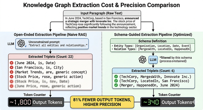
Schema-Guided vs. Open-Ended Extraction

綱要引導式提取 vs. 開放式提取

Optimization 2: Dual-Perception Community Detection / 優化二：雙重感知社群偵測 (Dual-Perception Community Detection)

Standard GraphRAG uses the Leiden algorithm for community detection — a purely topological approach that partitions the graph based on modularity optimization. This works, but it has a well-documented problem on knowledge graphs: there are often exponentially many near-optimal partitions, and purely structural methods can’t distinguish between them. Recent research has shown that Leiden-based community detection is unreliable on knowledge graphs for exactly this reason.

標準 GraphRAG 使用 Leiden 演算法進行社群偵測——這是一種純粹拓撲性 (Topological) 的方法，基於模組度優化 (Modularity Optimization) 來劃分圖。這方法行得通，但它在知識圖譜上有一個被充分記載的問題：往往存在指數級數量的近似最佳劃分，而純結構性方法無法區分它們。近期研究顯示，正是基於這個原因，基於 Leiden 的社群偵測在知識圖譜上並不可靠。

The fix is dual-perception community detection, which combines topological structure with semantic similarity. The scoring function for assigning an entity eᵢ to community Cₘ is:

解決之道是雙重感知社群偵測，它結合了拓撲結構與語義相似度 (Semantic Similarity)。將實體 eᵢ 指派至社群 Cₘ 的評分函式為：

φ(eᵢ, Cₘ) = α · Sᵣ(eᵢ, Cₘ) + (1 - α) · Sₛ(eᵢ, Cₘ)

Where:

其中：

• Sᵣ is the relational component: Jaccard similarity between the relations incident to eᵢ and those already in Cₘ

• Sᵣ 是 關係分量 (Relational Component)：與 eᵢ 相連的關係和 Cₘ 中已有關係之間的 Jaccard 相似度 (Jaccard Similarity)

• Sₛ is the semantic component: cosine similarity between the entity embedding of eᵢ and the centroid embedding of Cₘ

• Sₛ 是 語義分量 (Semantic Component)：eᵢ 的實體嵌入向量 (Embedding) 與 Cₘ 的質心嵌入向量 (Centroid Embedding) 之間的餘弦相似度 (Cosine Similarity)

• α balances the two (we use α = 0.6 in production, slightly favoring structure)

• α 用於平衡兩者（我們在生產環境中使用 α = 0.6，略微偏重結構）

The algorithm then performs iterative cluster fusion: clusters Cₐ and Cᵦ are merged if their dual-perception divergence falls below a threshold ε. This produces communities that are both structurally cohesive and semantically coherent.

接著，演算法執行迭代式叢集融合 (Iterative Cluster Fusion)：如果叢集 Cₐ 與 Cᵦ 的雙重感知散度 (Divergence) 低於閾值 ε，它們就會被合併。這會產生既在結構上凝聚、又在語義上連貫的社群。

def dual_perception_score(entity, community, alpha=0.6):  
    """Compute combined structural + semantic community affinity."""  
    # Relational: Jaccard similarity of relation types  
    entity_rels = set(get_relation_types(entity))  
    community_rels = set(get_relation_types_in_community(community))  
    jaccard = len(entity_rels & community_rels) / len(entity_rels | community_rels)    # Semantic: cosine similarity of embeddings  
    entity_emb = get_embedding(entity)  
    community_centroid = compute_centroid(community)  
    cosine_sim = np.dot(entity_emb, community_centroid) / (  
        np.linalg.norm(entity_emb) * np.linalg.norm(community_centroid)  
    )  
    return alpha * jaccard + (1 - alpha) * cosine_sim

Why does this matter for token costs? Because better communities mean better summaries, which in turn mean fewer irrelevant summaries are pulled into query-time context windows. When communities are noisy (mixing unrelated entities because they happen to be structurally adjacent), their summaries are unfocused, and the query-time map-reduce has to scan more of them to find relevant information. Clean communities → focused summaries → fewer summaries needed → fewer tokens.

這為什麼會影響 token 成本？因為更好的社群意味著更好的摘要，而更好的摘要又意味著被拉入查詢時上下文視窗的無關摘要更少。當社群充滿雜訊時（因為實體碰巧在結構上相鄰就被混在一起），它們的摘要便缺乏聚焦，查詢時的 map-reduce 就必須掃描更多摘要才能找到相關資訊。乾淨的社群 → 聚焦的摘要 → 所需摘要更少 → token 更少。

Optimization 3: The Four-Level Knowledge Tree / 優化三：四層知識樹 (Four-Level Knowledge Tree)

Instead of a flat graph with community overlays, the optimized architecture organizes knowledge into a four-level hierarchical tree:

優化後的架構並非採用帶有社群疊加的扁平圖，而是將知識組織成一棵四層的階層式樹：

 Level Contents                                                      Granularity       
------ ------------------------------------------------------------- ------------  
 L₁    Entity-attribute pairs (type + value)                         Finest            
 L₂    Entity-relation triplets `(head, relation, tail)`             Fine              
 L₃    Community keywords (highest-scoring entities per community)   Coarse            
 L₄    Community summaries (LLM-generated cluster descriptions)      Coarsest

Press enter or click to view image in full size

按下 Enter 鍵或點擊以檢視全尺寸圖片

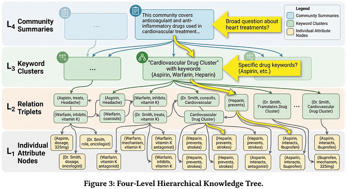
Four-Level Hierarchical Knowledge Tree

四層階層式知識樹

The key insight is that different queries need different levels. A factual lookup like “What is the dosage of Aspirin?” can be answered at L₁ without ever touching community summaries. A relational question like “What drugs treat Disease X?” resolves at L₂. A thematic question like “What are the main treatment approaches for cardiovascular disease?” routes to L₃/L₄.

關鍵洞見在於：不同的查詢需要不同的層級。像「阿斯匹靈的劑量是多少？」這樣的事實性查詢，可以在 L₁ 解決，完全不必觸及社群摘要。像「哪些藥物能治療疾病 X？」這樣的關係性問題，則在 L₂ 解決。像「心血管疾病的主要治療方法有哪些？」這樣的主題性 (Thematic) 問題，則被路由到 L₃/L₄。

This routing means you only pay for the granularity you need:

這種路由意味著你只需為你所需的粒度 (Granularity) 付費：

def route_query(query, schema):  
    """Route query to the appropriate knowledge tree level."""  
    query_type = classify_query(query, schema)  

    if query_type == "attribute_lookup":  
        # L1: Direct attribute retrieval, minimal tokens  
        return retrieve_attributes(query, level=1)  

    elif query_type == "relational":  
        # L2: Triple matching, moderate tokens  
        return retrieve_triples(query, level=2)  

    elif query_type == "thematic":  
        # L3+L4: Community-level, uses summaries  
        keywords = retrieve_keywords(query, level=3)  
        return retrieve_community_summaries(keywords, level=4)  

    elif query_type == "complex_multi_hop":  
        # Agentic decomposition (see next section)  
        return agentic_retrieve(query, all_levels=True)

In production, roughly 40% of our queries resolve at L₁ or L₂, never touching the expensive community summarization layer. That alone cuts average query-time token consumption nearly in half.

在生產環境中，我們大約 40% 的查詢在 L₁ 或 L₂ 就解決了，完全不必觸及昂貴的社群摘要層。光是這一點，就將平均查詢時的 token 消耗削減了近一半。

Optimization 4: Agentic Query Decomposition with Reflection / 優化四：帶反思的代理式查詢分解 (Agentic Query Decomposition with Reflection)

For the remaining 60% — the complex, multi-hop queries that are the whole reason you’re using GraphRAG in the first place — the agentic retriever decomposes them into parallel sub-queries that target specific schema elements.

對於剩下的 60%——那些複雜的、多跳的查詢，也正是你一開始使用 GraphRAG 的全部理由——代理式檢索器 (Agentic Retriever) 會將它們分解成針對特定綱要元素的平行子查詢 (Sub-query)。

The decomposition works by mapping query fragments to the schema types Sₑ, Sᵣ, and Sₐₜₜᵣ. A question like "Which organizations working on gene therapy have drugs in Phase III trials for rare diseases?" breaks down into:

這種分解的運作方式是將查詢片段對應到綱要類型 Sₑ、Sᵣ 和 Sₐₜₜᵣ。像 「哪些從事基因療法的組織，擁有正在進行罕見疾病第三期試驗的藥物？」 這樣的問題，會被拆解成：

1. Entity sub-query: Find entities of type Organization related to Gene Therapy

2. 實體子查詢： 尋找與 Gene Therapy（基因療法）相關、類型為 Organization（組織）的實體

3. Relation sub-query: Find (Drug, in_trial_for, Disease) triples where trial phase = III

4. 關係子查詢： 尋找試驗階段 = III 的 (Drug, in_trial_for, Disease) 三元組

5. Attribute sub-query: Filter diseases by rarity = rare

6. 屬性子查詢： 以 rarity = rare（罕見性 = 罕見）篩選疾病

7. Join: Intersect organizations across sub-query results

8. 聯結 (Join)： 對各子查詢結果中的組織取交集

Each sub-query targets one of four retrieval strategies:

每個子查詢都針對四種檢索策略中的一種：

# Strategy 1: Entity matching (node-level)  
entities = match_entities(sub_query, entity_type="Organization")  

# Strategy 2: Triple matching (edge-level)  
triples = match_triples(sub_query, relation_type="in_trial_for")  

# Strategy 3: Community filtering (cluster-level)  
communities = filter_communities(sub_query, keyword_threshold=0.7)  

# Strategy 4: DFS path traversal (multi-hop, max depth d=5)  
paths = dfs_traverse(start_entity, max_depth=5, relation_filter=schema.relations)

The reflection mechanism is the critical component that prevents the decomposition from under- or over-retrieving. After each retrieval round, the system evaluates completeness:

反思機制 (Reflection Mechanism) 是防止分解出現檢索不足或檢索過度的關鍵元件。在每一輪檢索之後，系統都會評估完整性：

Action(t) = f_llm( query[Reasoning], History(t-1)[Reflection] )

Where History maintains the chain of previous reasoning steps and retrieved results. If the reflection step identifies gaps ("We found the organizations but haven't confirmed which have Phase III drugs"), it generates targeted follow-up sub-queries. If it identifies redundancy ("Sub-queries 2 and 3 returned overlapping results"), it prunes.

其中 History 維護著先前推理步驟與檢索結果的鏈條。如果反思步驟識別出缺口（「我們找到了這些組織，但尚未確認哪些擁有第三期藥物」），它就會生成有針對性的後續子查詢。如果它識別出冗餘（「子查詢 2 和 3 回傳了重疊的結果」），它就會進行剪枝 (Prune)。

Press enter or click to view image in full size

按下 Enter 鍵或點擊以檢視全尺寸圖片

Agentic Query Decomposition with Reflection Loop

帶反思迴圈的代理式查詢分解

This is where token savings compound. Naive complex-query handling stuffs the entire relevant subgraph into a single massive context window — often 8,000–16,000 tokens of context for a single query. The agentic approach runs 3–5 focused sub-queries, each 200–500 tokens, plus a lightweight synthesis step. Total: 1,000–3,000 tokens for comparable or better accuracy.

這正是 token 節省效應疊加之處。樸素的複雜查詢處理會把整個相關子圖 (Subgraph) 塞進單一個龐大的上下文視窗——單一查詢往往就有 8,000 到 16,000 個 token 的上下文。代理式方法則運行 3 到 5 個聚焦的子查詢，每個 200 到 500 個 token，外加一個輕量的綜合步驟。總計：1,000 到 3,000 個 token，卻能達到相當或更好的準確率。

How Other Recent Approaches Compare / 其他近期方法的比較

We didn’t arrive at our architecture in a vacuum. The past year has produced a rich landscape of token-efficient GraphRAG methods, and understanding their trade-offs is essential for choosing the right approach.

我們的架構並非憑空而來。過去一年產生了豐富多樣的 token 高效 GraphRAG 方法，而理解它們之間的權衡取捨，對於選擇正確的方法至關重要。

KET-RAG: The Skeleton Strategy (KDD 2025) / KET-RAG：骨架策略 (KDD 2025)

KET-RAG asks: what if you only built a knowledge graph from the most important chunks?

KET-RAG 提出的問題是：如果你只從最重要的分塊來建立知識圖譜，會怎麼樣？

It identifies a small set of key text chunks (using TF-IDF and centrality heuristics) and runs full LLM-based extraction only on those. For everything else, it builds a lightweight text-keyword bipartite graph using deterministic NLP — no LLM required.

它識別出一小組關鍵文本分塊（使用 TF-IDF 與中心性 (Centrality) 啟發法），並只對這些分塊運行完整的、基於 LLM 的提取。對於其餘所有內容，它則使用確定性的 NLP 建立一個輕量的文本—關鍵字二部圖 (Bipartite Graph)——完全不需要 LLM。

Full corpus (N chunks)  
  ├── Key chunks (k << N) → Full KG extraction (LLM)  
  └── Remaining chunks (N-k) → Bipartite graph (NLP only)

During retrieval, it searches both structures in parallel: full graph traversal on the skeleton, and a mimicked search on the bipartite graph. The result is comparable or superior retrieval quality to full GraphRAG at over an order of magnitude lower indexing cost.

在檢索期間，它平行搜尋這兩種結構：在骨架上進行完整的圖遍歷，以及在二部圖上進行模擬搜尋。其結果是在索引成本低了超過一個數量級的情況下，檢索品質與完整 GraphRAG 相當或更優。

Trade-off: You’re betting that the key-chunk identification heuristic correctly identifies the information-dense portions of your corpus. For well-structured domains (legal, medical, technical), this works well. For loosely structured corpora (chat logs, social media), the heuristic may miss important information in “unimportant” chunks.

權衡取捨： 你是在賭關鍵分塊識別啟發法能正確地識別出語料庫中資訊密集的部分。對於結構良好的領域（法律、醫療、技術），這效果很好。對於結構鬆散的語料庫（聊天記錄、社群媒體），該啟發法可能會錯過藏在「不重要」分塊中的重要資訊。

TERAG: Aggressive Cost-Quality Trade-off (September 2025) / TERAG：激進的成本—品質權衡（2025 年 9 月）

TERAG replaces multi-hop LLM-based extraction with single-pass concept-level extraction and uses Personalized PageRank (PPR) during retrieval instead of LLM-based traversal:

TERAG 用單遍 (Single-pass) 的概念層級提取取代了多跳的、基於 LLM 的提取，並在檢索期間使用個人化網頁排名 (Personalized PageRank, PPR) 來取代基於 LLM 的遍歷：

# TERAG-style retrieval: PPR instead of LLM traversal  
def terag_retrieve(query, graph, damping=0.85, top_k=20):  
    seed_nodes = embed_and_match(query, graph.nodes)  
    ppr_scores = personalized_pagerank(  
        graph, seed_nodes, damping=damping  
    )  
    return sorted(ppr_scores.items(), key=lambda x: -x[1])[:top_k]

The numbers are striking: 80%+ of baseline accuracy at just 3–11% of the token cost. That’s a 10–30x cost reduction.

這些數字相當驚人：以僅僅 3% 到 11% 的 token 成本，達到基準 (Baseline) 準確率的 80% 以上。這是 10 到 30 倍的成本削減。

Trade-off: The drop in accuracy is real and measurable. On complex multi-hop questions, TERAG underperforms schema-guided approaches by 10–15 percentage points. Best suited for high-volume, lower-stakes retrieval where cost per query matters more than peak accuracy.

權衡取捨： 準確率的下降是真實且可量測的。在複雜的多跳問題上，TERAG 比綱要引導式方法落後 10 到 15 個百分點。最適合用於高流量、低風險的檢索場景，在這些場景中每次查詢的成本比峰值準確率更重要。

LinearRAG: Zero-Cost Graph Construction (ICLR 2026) / LinearRAG：零成本圖構建 (ICLR 2026)

LinearRAG eliminates LLM token costs entirely during graph construction. It builds a “Tri-Graph” — three interconnected layers (document, passage, entity) — using only lightweight NLP for entity extraction and semantic similarity for linking. No LLM calls at all during indexing.

LinearRAG 在圖構建期間完全消除了 LLM 的 token 成本。它建立一個「三重圖 (Tri-Graph)」——三個相互連接的層（文件、段落、實體）——僅使用輕量的 NLP 來進行實體提取，並用語義相似度來進行連結。在索引期間完全沒有任何 LLM 呼叫。

Retrieval uses a two-stage strategy:

檢索採用兩階段策略：

1. Local semantic bridging: Activate relevant entities via embedding similarity

2. 局部語義橋接 (Local Semantic Bridging)： 透過嵌入向量相似度來啟動相關實體

3. Global importance aggregation: Propagate importance scores through the Tri-Graph to rank passages

4. 全域重要性聚合 (Global Importance Aggregation)： 透過三重圖傳播重要性分數，以對段落進行排序

On the 2WikiMultiHopQA benchmark, LinearRAG achieves 70.20 Contain-Accuracy vs. 62.70 for HippoRAG2 and 48.60 for vanilla RAG — higher accuracy with zero additional indexing cost.

在 2WikiMultiHopQA 基準測試中，LinearRAG 達到了 70.20 的包含準確率 (Contain-Accuracy)，相較之下 HippoRAG2 為 62.70，而樸素 (Vanilla) RAG 為 48.60——在零額外索引成本的情況下達到了更高的準確率。

Trade-off: Without LLM-based extraction, the graph captures co-occurrence and similarity relationships but may miss nuanced, implicit relationships that only an LLM would infer. For domains where explicit relationships dominate (scientific literature, structured reports), this is fine. For domains with subtle, implied connections (legal reasoning, strategic analysis), LLM-based extraction still has an edge.

權衡取捨： 在沒有基於 LLM 的提取下，該圖能捕捉共現 (Co-occurrence) 與相似性關係，但可能會錯過那些只有 LLM 才能推斷出的、細微的隱含關係。對於顯式關係佔主導地位的領域（科學文獻、結構化報告），這沒問題。對於存在微妙、隱含連結的領域（法律推理、策略分析），基於 LLM 的提取仍然更具優勢。

LazyGraphRAG: Just-in-Time Graph Analysis (Microsoft Research) / LazyGraphRAG：即時圖分析（微軟研究院）

LazyGraphRAG takes the most radical position: build no graph summaries upfront. Index at the same cost as vanilla vector RAG (0.1% of full GraphRAG), and defer all LLM analysis to query time.

LazyGraphRAG 採取了最激進的立場：預先完全不建立任何圖摘要。以與樸素向量 RAG 相同的成本（完整 GraphRAG 的 0.1%）來建立索引，並將所有 LLM 分析延後到查詢時。

At query time, it combines vector search with a lightweight NLP-extracted graph structure, identifying relevant communities on the fly and generating summaries only for the specific communities needed to answer the current question.

在查詢時，它將向量搜尋與輕量的 NLP 提取圖結構結合起來，即時識別相關社群，並只為回答當前問題所需的特定社群生成摘要。

Trade-off: Query latency increases because summarization happens at query time rather than being pre-computed. For interactive applications where sub-second response times matter, this trade-off may not work. For batch processing or asynchronous workflows, it’s excellent.

權衡取捨： 查詢延遲 (Latency) 會增加，因為摘要是在查詢時進行的，而非預先計算。對於需要次秒級回應時間的互動式應用，這種權衡可能行不通。但對於批次處理或非同步 (Asynchronous) 工作流程，它則非常出色。

Clue-RAG: Multi-Granular Indexing (July 2025) / Clue-RAG：多粒度索引（2025 年 7 月）

Clue-RAG introduces a multi-partite graph with three node types — chunks, knowledge units, and entities — connected by typed edges. Its Q-Iter retrieval uses spreading activation with dynamic query embedding updates:

Clue-RAG 引入了一個多部圖 (Multi-partite Graph)，包含三種節點類型——分塊、知識單元 (Knowledge Unit) 與實體——並由具類型的邊 (Typed Edge) 連接。它的 Q-Iter 檢索使用帶有動態查詢嵌入向量更新的擴散激活 (Spreading Activation)：

# Clue-RAG style: iterative retrieval with spreading activation  
def q_iter_retrieve(query, graph, max_iterations=3):  
    query_embedding = encode(query)  
    activated = set()  

    for iteration in range(max_iterations):  
        # Anchor on entities + semantically similar knowledge units  
        new_nodes = spread_activation(query_embedding, graph, activated)  
        activated.update(new_nodes)  

        # Re-rank based on query-context coherence  
        activated = rerank(query_embedding, activated, graph)  

        # Update query embedding to avoid redundancy  
        query_embedding = update_query(query_embedding, activated)  

    return activated

Results: up to 99.33% higher accuracy and 113.51% higher F1 score than baselines, with a 72.58% reduction in indexing costs. Notably, it matches baselines even without using an LLM for indexing.

結果：相較於基準，準確率最高提升 99.33%，F1 分數最高提升 113.51%，同時索引成本降低 72.58%。值得注意的是，即使不使用 LLM 來建立索引，它的表現也能與基準相當。

HippoRAG 2: Neurobiologically Inspired Memory (ICML 2025) / HippoRAG 2：受神經生物學啟發的記憶 (ICML 2025)

HippoRAG 2 models RAG as analogous to human hippocampal memory. It builds a dual-node knowledge graph comprising passage and phrase nodes, enhanced with Personalized PageRank for retrieval. The key innovation is LLM-based triple filtering during indexing — it uses the LLM sparingly to validate and prune extracted triples rather than generate them from scratch.

HippoRAG 2 將 RAG 建模為類比於人類海馬迴 (Hippocampal) 記憶。它建立一個由段落節點與片語節點組成的雙節點知識圖譜，並以個人化網頁排名來增強檢索。其關鍵創新在於索引期間基於 LLM 的三元組過濾——它謹慎地使用 LLM 來驗證並剪枝已提取的三元組，而非從零開始生成它們。

Result: 7-point F1 gain over pure embedding retrievers on associative tasks, with significantly fewer LLM tokens than full GraphRAG during indexing.

結果：在聯想性任務上，相較於純嵌入向量檢索器，F1 分數提升 7 個百分點，同時在索引期間使用的 LLM token 比完整 GraphRAG 顯著更少。

Press enter or click to view image in full size

按下 Enter 鍵或點擊以檢視全尺寸圖片

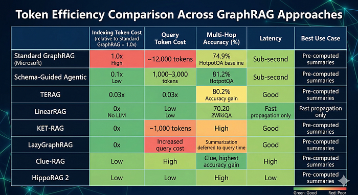
Token Efficiency Comparison Across GraphRAG Approaches

各種 GraphRAG 方法的 Token 效率比較

Anonymized Evaluation: Measuring What Actually Works / 匿名化評估：量測真正有效的東西

One thing that changed how we think about our pipeline was the adoption of anonymized evaluation. Here’s the problem: when you benchmark a GraphRAG system on a standard QA dataset, you can’t tell whether correct answers came from effective retrieval or from the LLM’s parametric knowledge. If GPT-4 already knows that “Aspirin treats headaches,” your retrieval pipeline gets credit it didn’t earn.

有一件事改變了我們對自己管線的思考方式，那就是採用了匿名化評估 (Anonymized Evaluation)。問題在於：當你在一個標準的問答 (QA) 資料集上對 GraphRAG 系統做基準測試時，你無法分辨正確答案究竟來自有效的檢索，還是來自 LLM 的參數化知識 (Parametric Knowledge)。如果 GPT-4 早就知道「阿斯匹靈能治療頭痛」，那麼你的檢索管線就獲得了它本不該得的功勞。

The AnonyRAG evaluation approach solves this by replacing entity mentions with opaque identifiers:

AnonyRAG 評估方法透過將實體提及替換為不透明的識別碼 (Opaque Identifier) 來解決這個問題：

Original:  "What drug does Company X use to treat Disease Y?"  
Anonymized: "What drug does [ORG#42] use to treat [DISEASE#17]?"

The LLM can’t answer from pre-trained knowledge because the entities are unrecognizable. It must rely entirely on retrieved evidence. This provides a much more honest measure of retrieval quality.

LLM 無法從預訓練知識中作答，因為這些實體無法辨識。它必須完全依賴檢索到的證據。這提供了一個對檢索品質更加誠實的量測。

When we switched to anonymized evaluation, several things we thought were working turned out to be parametric knowledge, and some retrieval improvements we’d dismissed as marginal turned out to be significant. It’s become a core part of our evaluation loop.

當我們改用匿名化評估後，有幾項我們以為有效的東西結果竟是參數化知識，而一些我們原本認為微不足道而不予理會的檢索改進，結果卻是顯著的。它已成為我們評估迴圈的核心部分。

def anonymize_dataset(dataset, entity_map=None):  
    """Replace named entities with opaque identifiers for fair evaluation."""  
    if entity_map is None:  
        entity_map = {}  
        counter = defaultdict(int)  
    anonymized = []  
    for item in dataset:  
        text = item["text"]  
        for entity, etype in extract_entities(text):  
            if entity not in entity_map:  
                counter[etype] += 1  
                entity_map[entity] = f"[{etype.upper()}#{counter[etype]}]"  
            text = text.replace(entity, entity_map[entity])  
        anonymized.append({**item, "text": text})  
    return anonymized, entity_map

Production Implementation Notes / 生產環境實作說明

A few practical details that don’t show up in papers but matter in production:

幾個不會出現在論文中、但在生產環境裡很重要的實務細節：

Schema versioning. As the schema expands automatically, you need to version it and track which graph nodes were extracted under which schema version. When you update the schema, you can selectively re-extract only the chunks that might contain entities matching new types, rather than rebuilding the entire graph.

綱要版本控制 (Schema Versioning)。 隨著綱要自動擴充，你需要為它建立版本，並追蹤哪些圖節點是在哪個綱要版本下提取的。當你更新綱要時，你可以選擇性地只重新提取那些可能包含符合新類型實體的分塊，而非重建整個圖。

@dataclass  
class SchemaVersion:  
    version: str  
    entity_types: Set[str]  
    relation_types: Set[str]  
    attribute_types: Set[str]  
    created_at: datetime  

    def diff(self, other: "SchemaVersion") -> SchemaDiff:  
        """Compute what changed between schema versions."""  
        return SchemaDiff(  
            new_entity_types=self.entity_types - other.entity_types,  
            new_relation_types=self.relation_types - other.relation_types,  
            new_attribute_types=self.attribute_types - other.attribute_types,  
        )

Community cache invalidation. When new documents are ingested and the graph changes, you don’t need to recompute all communities. Track which communities are affected by new edges and only regenerate summaries for those. This is similar to HIT-Leiden’s incremental approach—maintaining a hierarchical community structure and updating it through targeted movement, refinement, and aggregation phases rather than recomputing it from scratch.

社群快取失效 (Community Cache Invalidation)。 當新文件被攝入、圖發生變化時，你不需要重新計算所有社群。追蹤哪些社群受到新邊的影響，並只為那些社群重新生成摘要。這類似於 HIT-Leiden 的增量式 (Incremental) 方法——維護一個階層式社群結構，並透過有針對性的移動、精煉與聚合階段來更新它，而非從零開始重新計算。

Token budgeting per query. We set hard token budgets per query tier. Simple queries get a 500-token retrieval budget. Complex queries get 3,000. If the agentic decomposition’s reflection loop wants more, it has to justify it by demonstrating that previous rounds were insufficient — not by speculatively retrieving “just in case.”

每查詢 Token 預算編列。 我們為每個查詢層級設定硬性的 token 預算。簡單查詢獲得 500 個 token 的檢索預算。複雜查詢獲得 3,000 個。如果代理式分解的反思迴圈想要更多，它必須透過證明前幾輪檢索不足來提出正當理由——而不能「以防萬一」地投機性檢索。

Fallback to vector RAG. Not every query needs graph traversal. We run a lightweight classifier that routes ~25% of queries directly to vanilla vector RAG, bypassing the graph entirely. These are typically keyword-heavy factual lookups where vector similarity is sufficient. This hybrid routing is becoming standard across production GraphRAG systems.

回退至向量 RAG。 並非每個查詢都需要圖遍歷。我們運行一個輕量的分類器 (Classifier)，將約 25% 的查詢直接路由到樸素向量 RAG，完全繞過圖。這些通常是關鍵字密集的事實性查詢，向量相似度就足以應付。這種混合式路由 (Hybrid Routing) 正逐漸成為生產環境 GraphRAG 系統中的標準做法。

The Numbers / 數據

Here’s what these optimizations add up to in our production system:

以下是這些優化在我們生產系統中累積起來的成果：

Metric                          Standard GraphRAG   Our Architecture   Reduction        
------------------------------- ------------------- ------------------ ------------   
Indexing tokens (per 1K docs)   ~2.5M               ~230K              90.7%            
Avg. query tokens (simple)      ~2,800              ~450               84%              
Avg. query tokens (complex)     ~12,000             ~2,400             80%              
Monthly API cost (est.)         $14,200             $1,680             88%              
Multi-hop accuracy (HotpotQA)   74.9%               81.2%              +8.4%            
Multi-hop accuracy (2Wiki)      48.3%               77.6%              +60.7%

The accuracy improvements alongside cost reductions are the most compelling part of this story. It’s not a trade-off — structured, schema-guided extraction with hierarchical retrieval produces less noise in the context window, which translates directly to better answers.

準確率提升與成本削減並存，是這個故事最引人注目的部分。這並非一種權衡取捨——帶有階層式檢索的結構化、綱要引導式提取，能在上下文視窗中產生更少的雜訊，而這直接轉化為更好的答案。

Press enter or click to view image in full size

按下 Enter 鍵或點擊以檢視全尺寸圖片

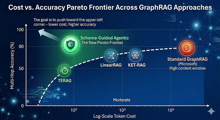
Cost vs. Accuracy Pareto Frontier Across GraphRAG Approaches

各種 GraphRAG 方法的成本 vs. 準確率帕雷托前緣 (Pareto Frontier)

Cost vs. Accuracy Pareto Frontier Across GraphRAG Approaches

各種 GraphRAG 方法的成本 vs. 準確率帕雷托前緣

Where This Is Heading / 趨勢走向

The trajectory from mid-2025 through early 2026 points clearly in a few directions.

從 2025 年中到 2026 年初的軌跡，清楚地指向幾個方向。

Hybrid routing as default architecture. Rather than one pipeline for all queries, production systems increasingly classify queries and route them to the appropriate retrieval strategy — vanilla vector for simple lookups, lightweight graph for relational queries, full agentic GraphRAG for complex multi-hop reasoning. The router itself is becoming a key piece of infrastructure.

混合式路由作為預設架構。 生產系統不再用單一管線處理所有查詢，而是愈來愈傾向對查詢進行分類，並將它們路由到合適的檢索策略——簡單查詢用樸素向量、關係性查詢用輕量圖、複雜的多跳推理用完整的代理式 GraphRAG。路由器本身正成為一項關鍵的基礎設施。

Incremental graph maintenance. Static, build-once graphs are giving way to continuously updated structures. HIT-Leiden, incremental community detection, and schema versioning are all pieces of a puzzle where the knowledge graph is a living structure that evolves with your corpus — not a snapshot that gets stale.

增量式圖維護。 靜態的、一次性構建的圖正讓位給持續更新的結構。HIT-Leiden、增量式社群偵測與綱要版本控制，都是同一幅拼圖的碎片——在這幅拼圖中，知識圖譜是一個隨語料庫演進的活結構，而非一張會過時的快照。

Deferred computation. LazyGraphRAG’s insight — don’t pre-compute what you might never need — is spreading. The next generation of production systems will likely pre-compute only the most frequently accessed graph regions and defer everything else to query time, using caching and pre-fetching heuristics to manage latency.

延後計算 (Deferred Computation)。 LazyGraphRAG 的洞見——別預先計算你可能永遠用不到的東西——正在擴散。下一代生產系統很可能只預先計算最常被存取的圖區域，並將其餘一切延後到查詢時，再用快取與預取 (Pre-fetching) 啟發法來管理延遲。

Token efficiency as first-class metric. With LLM API costs directly proportional to token consumption, and enterprise corpora measured in terabytes, the difference between a 90% reduction and a 50% reduction is millions of dollars per year. The frameworks that win in production will be the ones that treat tokens per correct answer as a primary optimization target — not an afterthought.

Token 效率作為一等指標。 由於 LLM API 成本與 token 消耗成正比，而企業語料庫的規模以 TB 計，90% 削減與 50% 削減之間的差異，每年就是數百萬美元。能在生產環境中勝出的框架，將會是那些把「每個正確答案所需 token 數」當作首要優化目標——而非事後才考慮——的框架。

The GraphRAG space has matured at a remarkable pace. What was an expensive research prototype eighteen months ago is now a diverse ecosystem of production-ready architectures, each optimizing a different point on the cost-quality-latency surface. The shared lesson across all of them: the best way to save tokens isn’t to use a cheaper model — it’s to structure your knowledge so that you need fewer tokens in the first place.

GraphRAG 領域以驚人的速度走向成熟。十八個月前還是個昂貴的研究原型，如今已是一個由多種可投入生產的架構組成的多元生態系，每一種都在成本—品質—延遲的曲面上優化著不同的點。它們共同的教訓是：節省 token 的最佳方式不是使用更便宜的模型——而是組織好你的知識，讓你從一開始就需要更少的 token。

References / 參考文獻

1. Dong et al., “Vertically Unified Agents for Graph Retrieval-Augmented Complex Reasoning,” arXiv:2508.19855, 2025. [ICLR 2026]

2. Dong 等人，〈用於圖檢索增強複雜推理的垂直統一代理〉，arXiv:2508.19855，2025 年。[ICLR 2026]

3. Xiao et al., “TERAG: Token-Efficient Graph-Based Retrieval-Augmented Generation,” arXiv:2509.18667, 2025.

4. Xiao 等人，〈TERAG：Token 高效的基於圖的檢索增強生成〉，arXiv:2509.18667，2025 年。

5. Zhuang et al., “LinearRAG: Linear Graph Retrieval Augmented Generation on Large-scale Corpora,” ICLR 2026.

6. Zhuang 等人，〈LinearRAG：大規模語料庫上的線性圖檢索增強生成〉，ICLR 2026。

7. Chen et al., “KET-RAG: A Cost-Efficient Multi-Granular Indexing Framework for Graph-RAG,” KDD 2025.

8. Chen 等人，〈KET-RAG：用於 Graph-RAG 的成本高效多粒度索引框架〉，KDD 2025。

9. Microsoft Research, “LazyGraphRAG: Setting a New Standard for Quality and Cost,” 2025.

10. 微軟研究院，〈LazyGraphRAG：為品質與成本樹立新標準〉，2025 年。

11. Guo et al., “LightRAG: Simple and Fast Retrieval-Augmented Generation,” EMNLP 2025.

12. Guo 等人，〈LightRAG：簡單且快速的檢索增強生成〉，EMNLP 2025。

13. Yin et al., “Clue-RAG: Towards Accurate and Cost-Efficient Graph-Based RAG via Multi-Partite Graph and Query-Driven Iterative Retrieval,” arXiv:2507.08445, 2025.

14. Yin 等人，〈Clue-RAG：透過多部圖與查詢驅動的迭代式檢索，邁向準確且成本高效的基於圖的 RAG〉，arXiv:2507.08445，2025 年。

15. Gutiérrez et al., “From RAG to Memory: Non-Parametric Continual Learning for Large Language Models” (HippoRAG 2), ICML 2025.

16. Gutiérrez 等人，〈從 RAG 到記憶：大型語言模型的非參數化持續學習〉（HippoRAG 2），ICML 2025。

17. Edge et al., “From Local to Global: A Graph RAG Approach to Query-Focused Summarization,” arXiv:2404.16130, 2024.

18. Edge 等人，〈從局部到全域：一種面向查詢摘要的 Graph RAG 方法〉，arXiv:2404.16130，2024 年。

---

🔤 關鍵術語

英文	繁中譯名	文章中的脈絡 / 簡短說明
GraphRAG	圖譜檢索增強生成	以知識圖譜為基礎的 RAG 架構，支援多跳推理與跨文件綜合，但 token 成本高
Schema-Guided Extraction	模式導向抽取	給 LLM 一個受限的實體／關係／屬性型別集合，輸出空間限縮為 Sₑ × Sᵣ × Sₑ，大幅減少抽取 token
Entity-Relation Triplet	實體─關係三元組	LLM 從文本抽取出的 (head, relation, tail) 結構，組裝成知識圖譜
Knowledge Graph	知識圖譜	由實體與關係三元組構成的圖結構，作為 RAG 檢索基礎
Community Detection	社群偵測	將圖譜分割為社群以利摘要；標準作法用 Leiden 演算法
Leiden Algorithm	Leiden 演算法	純拓樸式的模組度最佳化社群偵測，在知識圖譜上被指出不可靠
Dual-Perception Community Detection	雙重感知社群偵測	結合拓樸結構（Jaccard）與語意相似度（cosine）的社群分群評分函數
Jaccard Similarity	Jaccard 相似度	衡量實體與社群間關係型別重疊度的關係性成分 Sᵣ
Cosine Similarity	餘弦相似度	實體嵌入與社群中心嵌入間的語意成分 Sₛ
Entity Embedding	實體嵌入	實體的向量表示，用於計算語意相似度與社群中心
Hierarchical Knowledge Tree	階層式知識樹	四層架構（L₁ 屬性對、L₂ 三元組、L₃ 社群關鍵字、L₄ 社群摘要），按查詢需求路由粒度
Multi-Hop Reasoning	多跳推理	跨多個實體關係鏈進行的複雜查詢，是使用 GraphRAG 的核心動機
Agentic Query Decomposition	代理式查詢分解	將複雜查詢拆成針對 schema 元素的平行子查詢（實體／關係／屬性／join）
Reflection Mechanism	反思機制	每輪檢索後評估完整性，補齊缺口或裁剪冗餘的關鍵組件
DFS Path Traversal	深度優先路徑遍歷	多跳檢索策略之一，限制最大深度 d=5
Personalized PageRank (PPR)	個人化 PageRank	TERAG／HippoRAG 2 用以取代 LLM 遍歷的檢索演算法
Bipartite Graph	二部圖	KET-RAG 對非關鍵 chunk 以純 NLP 建立的輕量文字─關鍵字圖
Spreading Activation	擴散激活	Clue-RAG 的 Q-Iter 檢索機制，搭配動態查詢嵌入更新
Anonymized Evaluation (AnonyRAG)	匿名化評估	將實體換成不透明識別碼，避免 LLM 用參數化知識作答，公正衡量檢索品質
Parametric Knowledge	參數化知識	LLM 預訓練內含的知識，會使檢索效果評估失真
Hybrid Routing	混合路由	依查詢類型分流至 vector RAG／輕量圖／完整 agentic GraphRAG 的架構
Vector RAG	向量檢索增強生成	以向量相似度檢索的基礎 RAG，作為關鍵字型查詢的 fallback