為 1000 萬份以上文件打造近乎零幻覺的 RAG 管線
文章資訊
作者:Fareed Khan 日期:2026-07-03
原文標題:Building a RAG Pipeline for 10M+ Documents With Near-Zero Hallucination
📝 重點摘要
TL;DR
用檢索、約束、驗證、棄答四層防護,把不可答問題的幻覺率壓到 2%。
核心問題
語料規模擴大到千萬級時,RAG 生成模型在檢索落空時仍會「自信地編造」。本文不追求更聰明的模型,而是打造一套系統:當證據不足時,正確輸出是「棄答」而非流暢的猜測,同時檢索骨幹要能撐住 1000 萬向量並在毫秒內回應。
關鍵發現 / 數據
- 不可答的 100 題中棄答 98 題、僅答 2 題,幻覺率 2%(非零)。
- 已回答題的 faithfulness 0.908、context recall@k 0.97,但可答覆蓋率僅 0.46(安全的代價)。
- LanceDB IVF_PQ 索引在 1000 萬向量下 p95 僅 18.48ms,100 倍資料量延遲不到翻倍;外推至 1 億向量約 77.58ms、388GB。
- 驗證器在 HaluBench 上 AUROC 僅 0.702(優於隨機但遠非完美,是最大瓶頸)。
- 延遲以檢索為主(p50 3.07s),瓶頸是 LLM 呼叫而非向量搜尋。
方法亮點
- 混合檢索:Dense 向量(LanceDB)+ BM25,用 RRF 依排名融合(免分數正規化),150 候選重排到 20。
- 逐句引用生成:每句強制引用 passage id,並剝除模型捏造的假引用。
- 原子宣稱驗證閘:把答案拆成原子 claim,逐一用 32B judge 打分,取「最弱 claim」而非平均,任一不過即降級為棄答。
- CRAG 自我修正迴圈(LangGraph):先評估證據強度,弱則改寫查詢重檢索,最多 3 跳。
對我的研究有用嗎?
「棄答為一級輸出」與「claim 層級驗證取最弱環節」的設計,對 GraphRAG 中控制多跳推理幻覺很有參考價值;contextual chunking(為每個 chunk 加一句情境)提升召回的做法可直接借用。risk-coverage 曲線把幻覺/覆蓋率當可調旋鈕的框架,也適合套用在圖譜檢索的信心校準。
評語
工程實作紮實、可復現,值得一讀;但「近乎零幻覺」標題偏行銷——2% 非零、覆蓋率僅 46%,且 1000 萬向量測試用的是合成隨機向量(recall 僅 0.1),只證延遲不證檢索品質,需留意。
🌐 中英對照
Author: Fareed Khan Published: Source: https://levelup.gitconnected.com/building-a-rag-pipeline-for-10m-documents-with-near-zero-hallucination-788e4b5b7f25 Fetched: 2026-07-03T00:28:30.918855
作者:Fareed Khan 發布時間: 來源:https://levelup.gitconnected.com/building-a-rag-pipeline-for-10m-documents-with-near-zero-hallucination-788e4b5b7f25 擷取時間:2026-07-03T00:28:30.918855
Building a RAG Pipeline for 10M+ Documents With Near-Zero Hallucination / 為超過千萬份文件打造近乎零幻覺的 RAG 流程
Retrieve, constrain, verify, abstain / 檢索、約束、驗證、棄答
Read this story for free: link
免費閱讀本文: 連結
The more documents you put into a RAG system, the more ways it has to make things up, and as the corpus grows into the millions, toward 10M and beyond, that hallucination problem only gets worse. To keep answers trustworthy at that scale, you need a pipeline where the agent checks its own evidence and cites every claim it makes, the same idea behind the citations that Claude uses.
你在一套 RAG(檢索增強生成,Retrieval-Augmented Generation)系統中放進越多文件,它能夠捏造事物的途徑就越多;當語料庫(corpus)成長到數百萬、朝著一千萬乃至更多前進時,這個幻覺(hallucination)問題只會愈發嚴重。要在這種規模下維持答案的可信度,你需要一套流程:讓代理(agent)檢查它自己的證據,並為它提出的每一個主張標註引用來源——這正是 Claude 所使用的引用機制背後的相同理念。
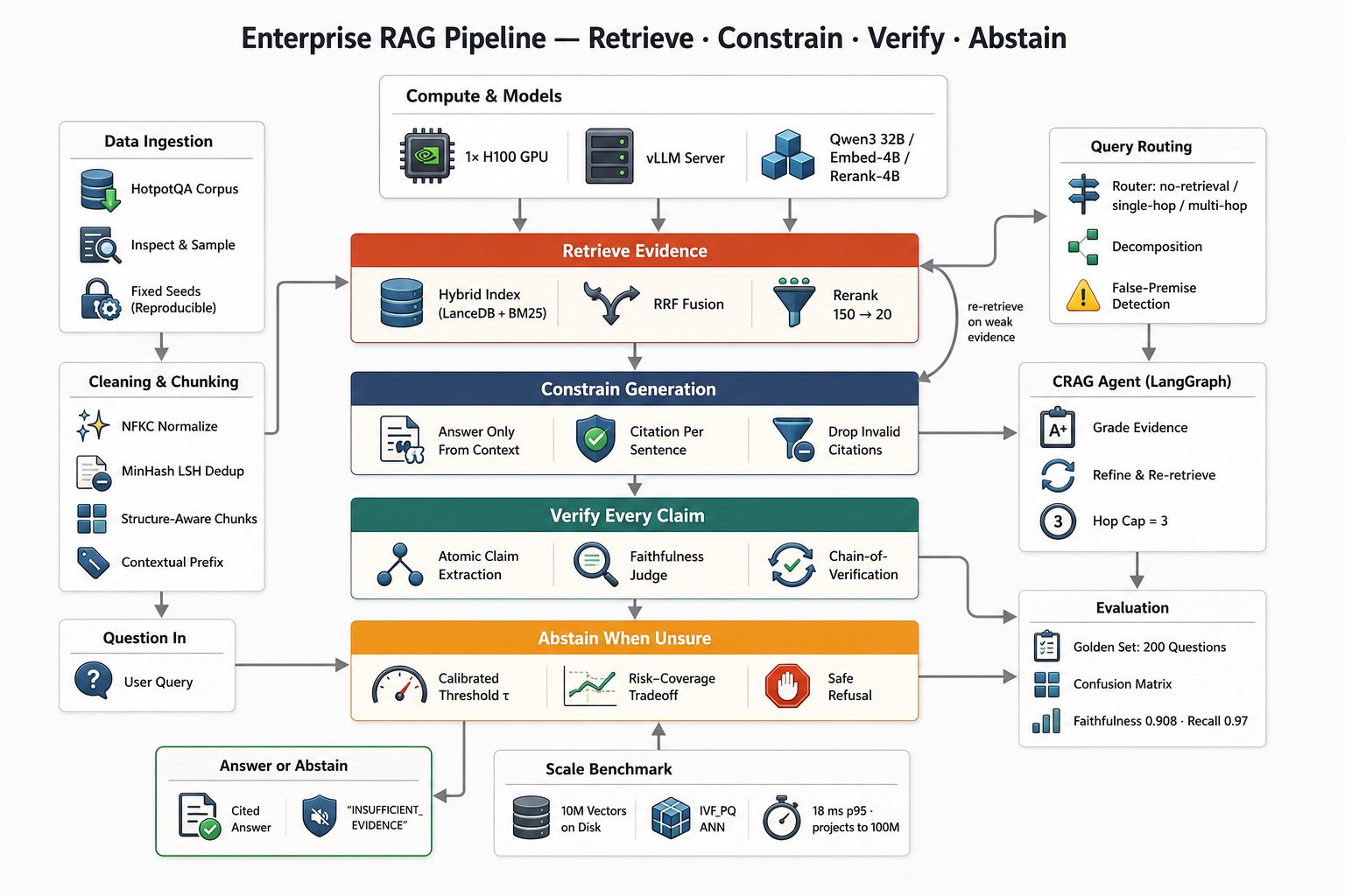
The full pipeline, from a question to a cited answer or a calibrated abstention (Created by
)
完整流程,從一個問題到帶有引用的答案,或是經過校準的棄答(abstention)(由
製作)
Here is everything the pipeline contains, and we build it top to bottom, one component at a time:
以下是這套流程所包含的一切,我們將由上而下、一次一個元件地把它建構起來:
- Set up and get the data: download the corpus, inspect its size and a real sample, and fix every seed so the run is reproducible.
-
設定並取得資料:下載語料庫,檢視它的規模與一份真實樣本,並固定每一個隨機種子(seed),讓整個執行可以重現。
-
Clean and chunk: normalize the text, drop near-duplicates with MinHash LSH, and cut it into structure-aware chunks with a one-line context prefix.
-
清理與切塊:正規化(normalize)文字,用 MinHash LSH 去除近似重複的內容,並將其切成具結構感知(structure-aware)的區塊(chunk),每塊前面加上一行情境前綴。
-
Build a hybrid index: store every chunk as a dense vector in LanceDB and a sparse BM25 posting, on disk so it scales to 10M+ vectors.
-
建立混合式索引:將每個區塊同時以稠密向量(dense vector)存進 LanceDB、以及以稀疏(sparse)BM25 倒排索引儲存,全部放在磁碟上,好讓它能擴展到超過一千萬個向量。
-
Retrieve and rerank: fuse the dense and sparse rankings with reciprocal rank fusion, then rerank 150 candidates down to 20.
-
檢索與重新排序:用倒數排名融合(Reciprocal Rank Fusion)把稠密與稀疏的排名結果融合起來,再將 150 個候選重新排序(rerank)精簡到 20 個。
-
Route and decompose: classify each question and split multi-hop ones into sub-questions before retrieving.
-
路由與分解:對每個問題進行分類,並在檢索之前把多跳(multi-hop)問題拆解成子問題。
-
Generate with citations: answer strictly from the context with a citation on every sentence, or emit an abstain token.
-
帶引用生成:嚴格根據上下文作答,每一句都附上引用,否則就輸出一個棄答標記(abstain token)。
-
Verify every claim: split the answer into atomic claims and check each one against its cited text with a faithfulness judge.
-
驗證每一個主張:把答案拆成原子級主張(atomic claim),並用一個忠實度評判者(faithfulness judge)逐一比對其所引用的文字。
-
Abstain when unsure: fold the signals into one calibrated decision and refuse when the support is not there.
-
不確定時就棄答:把各種訊號匯整成一個經過校準的決策,當支持證據不足時就拒絕回答。
-
Wire the agent: connect it all into a self-correcting CRAG loop that re-retrieves on weak evidence.
-
接上代理:把這一切連接成一個能自我修正的 CRAG(Corrective RAG,修正式 RAG)迴圈,在證據薄弱時重新檢索。
-
Evaluate and scale: score hallucination on a 200-question golden set, then benchmark the index to a real 10M vectors and project to 100M.
- 評估與擴展:在一組 200 題的黃金測試集(golden set)上評分幻覺率,接著把索引基準測試(benchmark)擴大到真實的一千萬個向量,並外推到一億。
All the code is available in my GitHub repository (Theory + Code):
所有程式碼都可在我的 GitHub 儲存庫中取得(理論+程式碼):
[## GitHub - FareedKhan-dev/rag-zero-hallucinations: Handling 10M+ docs using RAG with zero…
Handling 10M+ docs using RAG with zero hallucinatons - GitHub - FareedKhan-dev/rag-zero-hallucinations: Handling 10M+…
github.com](https://github.com/FareedKhan-dev/rag-zero-hallucinations?source=post_page-----788e4b5b7f25---------------------------------------)
[## GitHub - FareedKhan-dev/rag-zero-hallucinations:使用 RAG 處理超過千萬份文件並達到零幻覺……
使用 RAG 處理超過千萬份文件並達到零幻覺 - GitHub - FareedKhan-dev/rag-zero-hallucinations:Handling 10M+……
github.com](https://github.com/FareedKhan-dev/rag-zero-hallucinations?source=post_page-----788e4b5b7f25---------------------------------------)
Table of Contents / 目錄
- Near-Zero, Not Zero
- Setting Up the Project
- Getting the Data
- Cleaning the Corpus
- Chunking and Context
- Loading the Retrieval Models
- Building the Hybrid Index
- Retrieval: Fusion and Reranking ∘ Reciprocal rank fusion ∘ Reranking
- Routing and Decomposition
- Cited Generation
- The Verification Gate
- Knowing When to Abstain
- The Agent
- Does It Work? ∘ The golden set ∘ Hallucinations live in one cell ∘ The price of safety ∘ Is the judge any good?
- Scaling to 10M+ Vectors ∘ A real 10M-vector index ∘ 18 ms at ten million, and a 100M projection ∘ Where the time goes
- 設定專案
- 取得資料
- 清理語料庫
- 切塊與情境
- 載入檢索模型
- 建立混合式索引
- 檢索:融合與重新排序 ∘ 倒數排名融合 ∘ 重新排序
- 路由與分解
- 帶引用的生成
- 驗證關卡
- 懂得何時該棄答
- 代理
- 它真的有效嗎? ∘ 黃金測試集 ∘ 幻覺只住在一個格子裡 ∘ 安全的代價 ∘ 評判者夠好嗎?
- 擴展到超過一千萬個向量 ∘ 一個真實的一千萬向量索引 ∘ 一千萬時的 18 毫秒,以及一億的外推 ∘ 時間花在哪裡
- 適用範圍與接下來的方向
Near-Zero, Not Zero / 近乎零,而非真正的零
The problem we have to solve is not “make the model smarter.” A bigger model still guesses when retrieval comes back empty, because guessing is what generation does.
我們必須解決的問題並不是「把模型變得更聰明」。當檢索一無所獲時,更大的模型依然會用猜的,因為猜測正是生成(generation)在做的事。
So instead of chasing a perfect model, we wrap an ordinary one in a system that has only one safe failure mode. When the evidence is missing, the right output is not a fluent guess, it is an abstention.
因此,我們不去追求一個完美的模型,而是把一個平凡的模型包裹在一套只有唯一一種安全失敗模式的系統裡。當證據缺失時,正確的輸出不是一個流暢的猜測,而是棄答。
Press enter or click to view image in full size
按下 Enter 或點擊以檢視完整尺寸圖片

The rule the whole system follows: retrieve evidence, constrain generation to it, verify every claim, and abstain when support is missing (Created by
)
整套系統所遵循的規則:檢索證據、將生成約束在這些證據上、驗證每一個主張,並在支持不足時棄答(由
製作)
That gives us four control layers, and every section below is one of them.
這給了我們四個控制層,而下面的每一個小節都對應其中一層。
- Retrieve the right evidence: hybrid dense plus BM25 search, contextual chunks, and reranking.
-
檢索出正確的證據:混合式的稠密加上 BM25 搜尋、帶情境的區塊,以及重新排序。
-
Constrain generation: answer only from the context, cite passage ids for every sentence, or abstain.
-
約束生成:只根據上下文作答,為每一句標註段落 id 的引用,否則就棄答。
-
Verify every atomic claim: check each claim against the cited text with a faithfulness judge.
-
驗證每一個原子級主張:用忠實度評判者將每個主張與所引用的文字逐一比對。
-
Abstain: when claim support or retrieval confidence falls below a calibrated threshold.
- 棄答:當主張的支持度或檢索的信心低於一個經過校準的門檻(threshold)時。
We are after two goals at the same time. The first is trust, which means near-zero hallucination on the questions we choose to answer.
我們同時在追求兩個目標。第一個是信任,也就是在我們選擇回答的問題上達到近乎零的幻覺。
The second is scale, which means the retrieval backbone has to hold 10M+ vectors and still answer in milliseconds. The first goal needs the verification logic, the second needs the index.
第二個是規模,也就是檢索骨幹(backbone)必須能容納超過一千萬個向量,同時仍以毫秒為單位作答。第一個目標需要驗證邏輯,第二個目標需要索引。
We build both.
兩者我們都會建構。
Setting Up the Project / 設定專案
Before any of the logic, we set up the project. The plan is to import the libraries, fix every random seed so the run is reproducible, check the one GPU we are given, point a thin client at the generator, and freeze the config so a headless run behaves the same every time.
在任何邏輯之前,我們先把專案設定好。計畫是:匯入函式庫、固定每一個隨機種子讓執行可重現、檢查我們拿到的那一張 GPU、把一個精簡客戶端(thin client)指向生成器(generator),並凍結設定(config),好讓無介面(headless)的執行每次表現都一致。
Press enter or click to view image in full size
按下 Enter 或點擊以檢視完整尺寸圖片

Setup: import the libraries and seed, check the GPU, point a warm client at the generator, freeze the config (Created by
)
設定:匯入函式庫與種子、檢查 GPU、把一個熱備(warm)客戶端指向生成器、凍結設定(由
製作)
First the imports and a single function that seeds every random number generator we will touch.
首先是匯入,以及一個為我們會用到的每一個亂數產生器(random number generator)設定種子的函式。
import json, os, random, subprocess, time
from dataclasses import dataclass, asdict, field
import numpy as np


def set_determinism(seed: int) -> None:
    """Seed every RNG we touch so runs are reproducible."""
    random.seed(seed)
    np.random.seed(seed)
    os.environ["PYTHONHASHSEED"] = str(seed)
    try:
        import torch
        torch.manual_seed(seed)
        torch.cuda.manual_seed_all(seed)
    except Exception:
        pass


set_determinism(42)
I fix the seed up front because a RAG evaluation that is not reproducible is not an evaluation, and because the whole point of this blog is to trust the numbers at the end. The notebook is also parameterized, so one cell resolves the run profile and prints what we are about to build on.
我一開始就固定種子,因為一個無法重現的 RAG 評估根本稱不上是評估,也因為這整篇部落格的重點就是要能信任最後的數字。這個筆記本(notebook)也做了參數化,因此有一個儲存格會解析出執行設定檔(profile)並印出我們即將在其上建構的內容。
This is the full run, twenty thousand passages and a hundred plus a hundred evaluation questions, not the tiny smoke profile I use first to shake out code errors cheaply. We are on a single GPU, so VRAM is a hard budget, not a runtime surprise. We read the card with nvidia-smi and assert we are where we expect to be.
這是完整的執行,兩萬段文字(passage)加上一百外加一百題的評估問題,而不是我一開始用來廉價地揪出程式碼錯誤的那個極小型冒煙測試(smoke)設定檔。我們只用一張 GPU,所以 VRAM(顯示卡記憶體)是一個硬性的預算,而不是執行時才冒出來的意外。我們用 nvidia-smi 讀取這張卡,並斷言(assert)我們正處於預期的環境。
def gpu_report() -> dict:
    """Return GPU name / memory / driver and assert we are on an 80GB H100."""
    name = _smi("name")[0]
    total = float(_smi("memory.total")[0]) / 1024.0          # GiB
    rep = {"name": name, "total_gb": round(total, 1),
           "free_gb": round(float(_smi("memory.free")[0]) / 1024.0, 1),
           "driver": _smi("driver_version")[0]}
    print(json.dumps(rep, indent=2))
    assert "H100" in name and total >= 79      # one 80GB H100, nothing smaller
    return rep
#### OUTPUT ####
{
  "name": "NVIDIA H100 PCIe",
  "total_gb": 79.6,
  "free_gb": 32.8,
  "driver": "570.195.03"
}
We are on one NVIDIA H100 with 80 GB, and the host around it has 180 GB of RAM and a 750 GB NVMe disk, which matters later when the index grows. The 32B generator does not live in this notebook.
我們用的是一張 80 GB 的 NVIDIA H100,而環繞它的主機有 180 GB 的 RAM 以及一顆 750 GB 的 NVMe 磁碟,這在稍後索引成長時會很重要。那個 32B 的生成器並不住在這個筆記本裡。
It lives in a separate vLLM server, and we talk to it with a small OpenAI-compatible client. Keeping it warm in its own process means we can re-run this notebook many times without ever reloading it.
它住在一個獨立的 vLLM 伺服器裡,我們用一個小型、相容於 OpenAI 的客戶端與它溝通。讓它在自己的行程(process)中保持熱備狀態,意味著我們可以多次重新執行這個筆記本,卻永遠不必重新載入它。
class LocalLLM:
    """Thin client for the warm vLLM OpenAI-compatible server."""

    def __init__(self, endpoint: str, model: str, thinking: bool = False):
        self.endpoint, self.model, self.thinking = endpoint.rstrip("/"), model, thinking

    def chat(self, system: str, user: str, temperature: float = 0.0, max_tokens: int = 512) -> str:
        body = {"model": self.model, "temperature": temperature, "max_tokens": max_tokens,
                "messages": [{"role": "system", "content": system},
                             {"role": "user", "content": user}]}
        if not self.thinking:                   # Qwen3: skip the <think> trace for low latency
            body["chat_template_kwargs"] = {"enable_thinking": False}
        r = requests.post(f"{self.endpoint}/chat/completions", json=body, timeout=120)
        r.raise_for_status()
        return r.json()["choices"][0]["message"]["content"]


llm = LocalLLM("http://localhost:8000/v1", "Qwen/Qwen3-32B")
print(f"[llm] up={llm.is_up()}")
The server is up. The last setup step is to freeze every knob into one config object and print it, so the numbers driving the rest of the blog are all in one place.
伺服器已經運作。最後一個設定步驟是把每一個旋鈕(knob)都凍結進單一個設定物件並印出來,這樣驅動這篇部落格其餘部分的數字全都集中在一個地方。
#### OUTPUT ####
{
  "gen_model": "Qwen/Qwen3-32B",
  "embed_offline": "Qwen/Qwen3-Embedding-4B",
  "rerank_model": "Qwen/Qwen3-Reranker-4B",
  "chunk_tokens": 256, "chunk_overlap": 32,
  "retrieve_k": 150, "rerank_top_n": 20, "rrf_k": 60,
  "max_hops": 3, "crag_ok": 0.7, "crag_bad": 0.4,
  "tau_claim": 0.3, "tau_abstain": 0.3, "seed": 42
}
We retrieve 150 candidates, rerank down to 20, allow the agent up to 3 corrective hops, and set two support thresholds at 0.3 that we will calibrate later. The generator is Qwen3–32B, the embedder and reranker are the 4B Qwen3 models, and the faithfulness judge is the 32B itself.
我們檢索 150 個候選、重新排序精簡到 20 個、允許代理最多做 3 次修正跳躍(corrective hop),並把兩個支持度門檻設在 0.3,稍後會加以校準。生成器是 Qwen3–32B,嵌入器(embedder)與重新排序器(reranker)是 4B 的 Qwen3 模型,而忠實度評判者就是那個 32B 本身。
I keep the generator at temperature 0 with the thinking trace off, because I want reproducible, low-latency answers, and because sampling is one more place a model can drift away from the evidence I gave it. Every model here is a local open-weight Qwen3, which I have to do because the entire premise is that no document and no query leaves this machine, which is exactly what makes a pipeline like this usable on a private corpus.
我讓生成器維持在溫度(temperature)0、關閉思考軌跡(thinking trace),因為我想要可重現、低延遲的答案,也因為取樣(sampling)是模型會偏離我所給證據的另一個地方。這裡的每一個模型都是本地端、開放權重(open-weight)的 Qwen3,我必須這麼做,因為整個前提就是沒有任何文件、沒有任何查詢會離開這台機器——而這正是讓像這樣的一套流程能夠用在私有語料庫上的關鍵。
With the tools ready, we can go get some data.
工具都備妥後,我們就可以去取得一些資料了。
Getting the Data / 取得資料
A pipeline is only as good as the corpus under it, so the first real step is to download a dataset and look at it. I went with HotpotQA in its distractor setting for two reasons.
一套流程的好壞取決於底下的語料庫,所以第一個真正的步驟是下載一個資料集並仔細看看它。我選了干擾項(distractor)設定下的 HotpotQA,有兩個原因。
Every question ships with sentence-level gold supporting facts, which is the cleanest way to score retrieval recall later, and its bundled Wikipedia paragraphs give me a real corpus for free. For the other side of the test I pull SQuAD v2 impossible questions and hand-write a handful of false-premise questions, because the only way to measure hallucination is to ask things the corpus cannot answer and check that the system stays quiet.
每一個問題都附帶句子層級的黃金支持事實(gold supporting fact),這是稍後為檢索召回率(recall)評分最乾淨的方式,而它所捆綁的維基百科段落免費給了我一個真實的語料庫。至於測試的另一面,我抽取 SQuAD v2 的無解問題,並手寫少量的假前提(false-premise)問題,因為衡量幻覺的唯一辦法,就是去問語料庫無法回答的東西,並檢查系統是否保持沉默。
A third set, HaluBench, comes in near the end purely to validate the verifier itself. HotpotQA is the corpus we build and search.
第三組資料集 HaluBench 在接近尾聲時登場,純粹是為了驗證驗證器(verifier)本身。HotpotQA 才是我們建構並搜尋的語料庫。
Press enter or click to view image in full size
按下 Enter 或點擊以檢視完整尺寸圖片
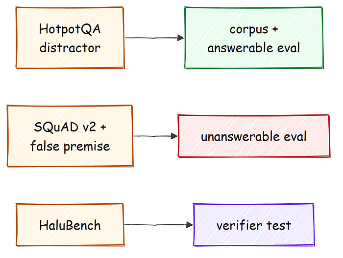
Each dataset has a role: HotpotQA is the corpus and answerable set, SQuAD v2 plus false premises are the unanswerable set, HaluBench tests the verifier (Created by
)
每個資料集都有其角色:HotpotQA 是語料庫與可回答集,SQuAD v2 加上假前提是不可回答集,HaluBench 則測試驗證器(由
製作)
from datasets import load_dataset

def load_hotpotqa(split: str = "validation"):
    # datasets 3.x wants the namespaced repo id
    return load_dataset("hotpotqa/hotpot_qa", "distractor", split=split, cache_dir=DS_CACHE)

hotpot = load_hotpotqa()
print(f"[data] hotpotqa(validation) = {len(hotpot)} questions")
That is 7,405 questions, and bundled with each one are the Wikipedia paragraphs it was drawn from. We define what a passage and a question look like, then a builder that unions every question’s context paragraphs into a corpus while keeping track of which passages are gold evidence.
那是 7,405 個問題,每一個都捆綁著它所取材的維基百科段落。我們先定義段落與問題長什麼樣子,接著定義一個建構器(builder),把每個問題的上下文段落聯集成一個語料庫,同時追蹤哪些段落屬於黃金證據。
@dataclass
class Passage:
    id: str
    title: str
    text: str
    is_gold_for: list[str] = field(default_factory=list)   # question ids this is gold for

@dataclass
class QAItem:
    qid: str
    question: str
    answer: str
    answerable: bool
    gold_titles: list[str] = field(default_factory=list)
    gold_sentences: list[str] = field(default_factory=list)
    qtype: str = ""    # bridge | comparison | unanswerable | false_premise
class CorpusBuilder:
    """Build a passage corpus + QA items from HotpotQA distractor contexts."""

    def build(self, qa, n_passages: int):
        passages, qa_items = {}, []
        for ex in qa:
            gold = list(dict.fromkeys(ex["supporting_facts"]["title"]))   # gold evidence titles
            for t, ss in zip(ex["context"]["title"], ex["context"]["sentences"]):
                para = " ".join(s.strip() for s in ss).strip()
                if len(para) < 40:
                    continue
                p = passages.setdefault(_pid(t, 0), Passage(_pid(t, 0), t, para))
                if t in gold:
                    p.is_gold_for.append(ex["id"])
            # (the full builder also records each question's gold supporting sentences)
            qa_items.append(QAItem(ex["id"], ex["question"], ex["answer"], True,
                                   gold_titles=gold, qtype=ex.get("type", "")))
            if len(passages) >= n_passages:
                break
        return list(passages.values()), qa_items

corpus, qa_items = CorpusBuilder().build(hotpot, SLICE_SIZE)
print(f"[corpus] passages={len(corpus)}  qa_items={len(qa_items)}  "
      f"gold-bearing passages={sum(1 for p in corpus if p.is_gold_for)}")
We now hold 20,007 passages and 2,073 questions, with 4,072 passages marked as gold evidence for some question. Before building anything on top of it, we should actually look at the data, both the size distribution and one real example.
我們現在握有 20,007 段文字與 2,073 個問題,其中有 4,072 段被標記為某個問題的黃金證據。在其上建構任何東西之前,我們應該實際看看資料,包含大小的分布以及一個真實的範例。
import pandas as pd

tok_lens = [len(p.text.split()) for p in corpus]
print(pd.Series(tok_lens, name="passage_word_count").describe().round(1).to_string())

ex = qa_items[0]
print(f"\nSample question:\n  Q: {ex.question}\n  A: {ex.answer}   (type={ex.qtype})")
print(f"  gold titles: {ex.gold_titles}")
for s in ex.gold_sentences:
    print(f"   - {s}")
#### OUTPUT ####
count    20007.0
mean        89.2
std         53.4
min          7.0
25%         54.0
50%         80.0
75%        113.0
max       1378.0

Sample question:
  Q: Were Scott Derrickson and Ed Wood of the same nationality?
  A: yes   (type=comparison)
  gold titles: ['Scott Derrickson', 'Ed Wood']
   - Scott Derrickson (born July 16, 1966) is an American director, screenwriter and producer.
   - Edward Davis Wood Jr. was an American filmmaker, actor, writer, producer, and director.
Passages run about 89 words on average, short enough that a couple fit in a prompt and long enough to carry a fact. The sample is a comparison question, “Were Scott Derrickson and Ed Wood of the same nationality?”, and its two gold sentences already contain the answer, that both men were American.
段落平均約 89 個字,短到足以讓兩三段塞進一則提示(prompt),又長到足以承載一個事實。這個範例是一個比較型問題「Scott Derrickson 和 Ed Wood 是同一個國籍嗎?」,而它的兩句黃金句子已經包含了答案,也就是這兩人都是美國人。
This is the question we will follow through every stage of the blog, because watching one real question travel the whole pipeline makes each component concrete. The two strata are already visible here.
這正是我們會貫穿整篇部落格每一個階段所追蹤的問題,因為看著一個真實問題走完整套流程,能讓每個元件變得具體。兩個層別(strata)在這裡已經看得出來了。
Answerable questions like this one let me measure whether the right evidence comes back, and the unanswerable questions I add later are how I measure hallucination, because a system that answers a question with no support in the corpus is a system that makes things up.
像這樣的可回答問題讓我能衡量正確的證據是否被檢索回來,而我稍後加入的不可回答問題,則是我衡量幻覺的方式,因為一套在語料庫中毫無支持卻仍回答問題的系統,就是一套在捏造事物的系統。
Cleaning the Corpus / 清理語料庫
Garbage in means hallucinations out, so before we index anything we clean the text. Two cheap steps pay off out of proportion. Normalization makes the tokenizer behave the same on every passage, and near-duplicate removal stops copied or forwarded passages from crowding the top results and inflating retrieval without adding any new evidence.
垃圾進,幻覺出,所以在索引任何東西之前,我們先清理文字。兩個成本低廉的步驟能帶來不成比例的回報。正規化讓分詞器(tokenizer)在每一段文字上都表現一致,而近似重複的移除則能阻止被複製或轉發的段落擠爆頂端結果、在不新增任何證據的情況下虛胖了檢索。
Press enter or click to view image in full size
按下 Enter 或點擊以檢視完整尺寸圖片

Cleaning: normalize every passage, then drop near-duplicates with MinHash LSH, leaving 19,987 passages (Created by
)
清理:正規化每一段文字,接著用 MinHash LSH 去除近似重複,留下 19,987 段文字(由
製作)
import re, unicodedata
def normalize_text(s: str) -> str:
s = unicodedata.normalize("NFKC", s) # canonical unicode form
s = s.replace("", "") # drop soft hyphens
s = re.sub(r"[ \t]+", " ", s) # collapse runs of spaces
return s.strip()
I run NFKC normalization first because BM25 tokenizes on raw characters, so a ligature or a run of stray spaces would split one word into two or merge two into one, and quietly hurt recall. On a messy string the function does exactly what we want.
我先執行 NFKC 正規化,因為 BM25 是在原始字元上分詞,所以一個連字(ligature)或一連串多餘的空格,會把一個字拆成兩個、或把兩個併成一個,並悄悄地傷害召回率。對一個雜亂的字串,這個函式做的正是我們想要的。
The ligature “fi” becomes a plain “fi” and the tab and runs of spaces collapse to single spaces, so two passages that differ only in invisible characters now tokenize identically.
連字「fi」變成了普通的「fi」,定位符(tab)與一連串空格都塌縮成單一空格,因此兩段只在不可見字元上有差異的文字,現在分詞的結果完全相同。
The deduper is the interesting part. I have to choose an approximate method like MinHash LSH rather than comparing every pair, because exact pairwise comparison is quadratic and would never finish at corpus scale, while MinHash with an LSH index finds near-duplicates in roughly linear time.
去重器(deduper)才是有趣的部分。我必須選擇像 MinHash LSH 這樣的近似方法,而不是比較每一對,因為精確的成對比較是平方級(quadratic)的,在語料庫規模下永遠跑不完;而搭配 LSH 索引的 MinHash 大約能以線性時間找出近似重複。
Dropping them serves both goals at once. It keeps the index smaller as we head toward 10M vectors, and it stops three copies of one paragraph from crowding the top results, which is a quiet way a retriever feeds the model redundant context and tempts it to over-trust a single source.
丟掉它們同時服務了兩個目標。當我們朝一千萬個向量前進時,這讓索引維持較小,同時它也阻止同一段落的三份拷貝擠爆頂端結果——那正是檢索器悄悄地餵給模型冗餘上下文、誘使它過度信任單一來源的一種方式。
class Deduper:
    """Drop near-duplicate passages via MinHash LSH over word shingles."""

    def __init__(self, threshold: float = 0.9, num_perm: int = 64):
        self.threshold, self.num_perm = threshold, num_perm

    def fit_transform(self, passages: list[Passage]):
        lsh = MinHashLSH(threshold=self.threshold, num_perm=self.num_perm)
        kept, dropped = [], 0
        for p in passages:
            m = self._mh(p.text)
            if lsh.query(m):              # a near-duplicate is already kept
                dropped += 1
                continue
            lsh.insert(p.id, m)
            kept.append(p)
        return kept, {"kept": len(kept), "dropped_near_dup": dropped}
#### OUTPUT ####
{
  "kept": 19987,
  "dropped_near_dup": 19,
  "input": 20007,
  "after_quality": 20006,
  "after_dedup": 19987
}
We keep 19,987 passages after dropping 19 near-duplicates and one short fragment. This corpus is a curated slice, but the cleaning step is exactly what you run unchanged whether the input is twenty thousand passages or twenty million.
在丟掉 19 段近似重複與一段短碎片後,我們留下 19,987 段文字。這個語料庫是一份精選的切片,但無論輸入是兩萬段或兩千萬段,你所執行的清理步驟都一模一樣、原封不動。
Chunking and Context / 切塊與情境
Now we cut passages into chunks. Fixed-size chunking is the easy choice and the wrong one, because it cuts an entity-bearing sentence away from the context that disambiguates it, which is fatal for multi-hop questions.
現在我們把段落切成區塊。固定大小的切塊是容易的選擇,卻是錯誤的選擇,因為它會把一個承載實體(entity)的句子從讓它得以消歧(disambiguate)的上下文中切開,這對多跳問題而言是致命的。
So we pack whole sentences up to a token budget with a small overlap, and we count tokens with the generator’s own tokenizer so the budget matches what the model will actually see. This is a hallucination problem hiding inside a chunking detail.
因此我們把完整的句子塞到一個 token 預算為止,並帶有小幅重疊(overlap),而且我們用生成器自己的分詞器來計算 token,好讓這個預算符合模型實際上會看到的內容。這是一個藏在切塊細節裡的幻覺問題。
If a chunk overflows the budget and gets silently truncated, the one sentence that held the answer can vanish, and the question then looks unanswerable for no real reason, so I would rather respect sentence boundaries and pay for a few extra chunks.
如果一個區塊超出預算而被悄悄截斷(truncate),那句握著答案的句子就可能消失,於是這個問題就毫無真正理由地看似不可回答,所以我寧可尊重句子的邊界,並為多出來的幾個區塊付出代價。
Press enter or click to view image in full size
按下 Enter 或點擊以檢視完整尺寸圖片

Chunking packs whole sentences to a token budget, then the contextualizer prepends a one-line situating sentence (Created by
)
切塊把完整句子塞到一個 token 預算內,接著情境化器(contextualizer)在前面加上一行定位用的句子(由
製作)
class StructureAwareChunker:
    def __init__(self, tokenizer, target_tokens: int = 256, overlap: int = 32):
        self.tok, self.target, self.overlap = tokenizer, target_tokens, overlap

    def chunk(self, passage: Passage) -> list[Chunk]:
        sents = split_sentences(passage.text) or [passage.text]
        chunks, cur, cur_tok = [], [], 0
        for s in sents:
            st = self._ntok(s)
            # start a new chunk once adding this sentence would blow the token budget
            if cur and cur_tok + st > self.target:
                chunks.append(self._make(passage, cur))
                # carry the trailing sentence forward so chunks overlap
                cur, cur_tok = ([cur[-1]], self._ntok(cur[-1])) if self.overlap else ([], 0)
            cur.append(s)
            cur_tok += st
        if cur:
            chunks.append(self._make(passage, cur))
        return chunks
That gives us 21,259 chunks at a mean of 125 tokens, comfortably under the 256 budget. There is one more problem to solve before indexing.
這給了我們 21,259 個區塊,平均 125 個 token,舒服地落在 256 的預算之下。在索引之前還有一個問題要解決。
A chunk like “revenue grew 3 percent that quarter” is unsearchable on its own, because whose revenue and which quarter are gone. So we prepend a one-line situating sentence to each chunk before indexing, which is the contextual retrieval idea, except we write that sentence with our local Qwen3 instead of a hosted model.
像「那一季營收成長了 3%」這樣的區塊本身是無法被搜尋的,因為「誰的營收」和「哪一季」都不見了。所以我們在索引之前,為每個區塊前面加上一行定位用的句子,這就是情境式檢索(contextual retrieval)的理念,只不過我們是用本地端的 Qwen3、而非託管(hosted)模型來寫這句話。
CONTEXTUALIZE_PROMPT = (
    "Here is a document titled '{title}':\n<document>\n{doc}\n</document>\n\n"
    "Here is a chunk from it:\n<chunk>\n{chunk}\n</chunk>\n\n"
    "Give a short, single-sentence context (<=25 words) that situates this chunk "
    "within the document so it can be retrieved on its own. Answer with the sentence only."
)
The method fans the per-chunk calls out across a thread pool, because the calls are independent and vLLM batches them server-side, which makes this far faster than going one chunk at a time. We also checkpoint the result so a rerun skips this whole step.
這個方法把每個區塊的呼叫展開(fan out)到一個執行緒池(thread pool)上,因為這些呼叫彼此獨立,而 vLLM 會在伺服器端把它們批次處理(batch),這讓它遠比一次一個區塊快得多。我們也為結果建立檢查點(checkpoint),好讓重新執行時能跳過這整個步驟。
class Contextualizer:
    def contextualize(self, chunks, doc_lookup, workers: int = 32):
        def _one(c):
            user = CONTEXTUALIZE_PROMPT.format(title=c.title,
                                               doc=doc_lookup.get(c.passage_id, c.text)[:4000],
                                               chunk=c.text)
            ctx = self.llm.chat("You write concise retrieval context.", user, max_tokens=64).strip()
            c.contextual_text = (ctx + "\n" + c.text) if ctx else c.text   # prefix, keep original
        with ThreadPoolExecutor(max_workers=workers) as ex:
            list(ex.map(_one, chunks))      # 32 in flight at once
        return chunks
#### OUTPUT ####
Before:
  Ed Wood is a 1994 American biographical period comedy-drama film directed and
  produced by Tim Burton, and starring Johnny Depp as cult filmmaker Ed Wood...

After (context-prefixed):
  This chunk introduces the 1994 film *Ed Wood*, directed by Tim Burton, and
  outlines its main subject and cast.
  Ed Wood is a 1994 American biographical period comedy-drama film...
The extra sentence is cheap, one short generation per chunk, and it tells the retriever what this chunk is about even when the chunk text alone would be ambiguous. That lift is most of why recall ends up so high. Recall is the foundation of the whole hallucination story, because the verifier downstream can only ground an answer in evidence that retrieval actually found, so every point of recall I buy here is a question I get to answer instead of refuse.
這句額外的句子成本低廉,每個區塊只要一次短短的生成,而且即使區塊文字本身會有歧義,它也能告訴檢索器這個區塊在講什麼。那份提升就是召回率最終如此之高的主要原因。召回率是整個幻覺故事的基礎,因為下游的驗證器只能把答案建立在檢索實際找到的證據上,所以我在這裡買到的每一分召回率,都是一個我得以回答、而非拒絕的問題。
Loading the Retrieval Models / 載入檢索模型
With the chunks ready, we load the models that turn them into searchable evidence and later check the answers. Three models share this GPU alongside the generator, so we snapshot VRAM after each load and stay under budget. We load the reranker and the faithfulness judge here, and the embedder a little later, only when we build the index.
區塊備妥後,我們載入那些把它們變成可搜尋證據、並在稍後檢查答案的模型。有三個模型和生成器一起共用這張 GPU,所以我們在每次載入後為 VRAM 拍快照(snapshot)並維持在預算之下。我們在這裡載入重新排序器與忠實度評判者,至於嵌入器則稍晚、只在建立索引時才載入。
Press enter or click to view image in full size
按下 Enter 或點擊以檢視完整尺寸圖片

One H100 holds the 32B generator in vLLM plus the embedder, reranker, and judge in the kernel (Created by
)
一張 H100 在 vLLM 中裝著 32B 生成器,外加在核心(kernel)中的嵌入器、重新排序器與評判者(由
製作)
We do not want to discover an overrun as an out-of-memory crash three steps later, so each load logs the whole-GPU number from nvidia-smi and the kernel-only number from torch.
我們不想在三個步驟之後才以記憶體不足(out-of-memory)當機的形式發現超用,所以每次載入都會記錄來自 nvidia-smi 的整張 GPU 數字,以及來自 torch 的僅核心(kernel-only)數字。
def vram_snapshot(tag: str) -> dict:
    """Log GPU-wide and kernel-only VRAM after each load step."""
    kernel = round(torch.cuda.memory_allocated() / 1024**3, 2)     # this kernel only
    used = round(float(_smi("memory.used")[0]) / 1024.0, 2)        # whole GPU, both processes
    print(f"[vram] {tag:22} gpu_used={used}GB  kernel={kernel}GB")
    return {"tag": tag, "gpu_used_gb": used, "kernel_gb": kernel}
The reranker is a small causal model used as a yes-or-no judge. Each query and document pair is wrapped in a fixed template, and the score is read straight from the next-token logits, so reranking is one forward pass per candidate. I load a dedicated cross-encoder reranker instead of trusting the embedding scores because the embedder compresses a whole passage into one vector, which is fast enough to scan the corpus but blurs the difference between a passage that merely mentions the entities and one that actually answers the question, and that difference is precisely what keeps the wrong evidence out of the prompt and out of the answer.
重新排序器是一個小型的因果(causal)模型,被當作一個是非題評判者來用。每一對查詢與文件都被包進一個固定模板裡,而分數直接從下一個 token 的 logits 讀出,所以重新排序對每個候選就是一次前向傳遞(forward pass)。我載入一個專門的交叉編碼器(cross-encoder)重新排序器,而不是信任嵌入分數,因為嵌入器把整段文字壓縮成一個向量,這快到足以掃描語料庫,卻模糊了「只是提到那些實體的段落」與「真正回答問題的段落」之間的差別,而這個差別,正是讓錯誤證據不進入提示、不進入答案的關鍵。
class Qwen3Reranker:
    """Scores a (query, doc) pair by the probability the model puts on the 'yes' token."""

    @torch.no_grad()
    def score(self, query: str, docs: list[str], batch_size: int = 16) -> list[float]:
        out = []
        for i in range(0, len(docs), batch_size):
            batch = [self._fmt(query, d) for d in docs[i:i + batch_size]]
            enc = self.tok(batch, return_tensors="pt", padding=True,
                           truncation=True, max_length=1024).to(self.model.device)
            logits = self.model(**enc).logits[:, -1, :]       # last-token logits
            yn = logits[:, [self.no_id, self.yes_id]]         # compare 'no' against 'yes'
            probs = torch.softmax(yn.float(), dim=-1)[:, 1]   # keep P('yes')
            out.extend(probs.cpu().tolist())
        return out
The faithfulness judge is the 32B generator itself, prompted to return a single support score for a claim against some context. I made the judge the local 32B because faithfulness checking in RAG means reading one claim against several long passages at once, which is exactly where a small sentence-pair NLI model gets brittle, and because this judge is the single component that turns a confident wrong answer into an abstention.
忠實度評判者就是那個 32B 生成器本身,被提示去針對某段上下文為一個主張回傳單一的支持分數。我讓評判者用本地端的 32B,因為 RAG 中的忠實度檢查意味著要一次把一個主張對照數段長文字來讀,而那正是小型的句對 NLI(自然語言推論,Natural Language Inference)模型會變得脆弱的地方,也因為這個評判者是把一個自信的錯誤答案轉成棄答的那唯一一個元件。
It is the heart of the near-zero hallucination claim, so I would rather spend the strongest model I have on it. An NLI cross-encoder and MiniCheck are still wired in as lighter alternatives, but this run uses the LLM judge.
它是近乎零幻覺這項主張的核心,所以我寧可把我手上最強的模型花在它身上。一個 NLI 交叉編碼器與 MiniCheck 仍然被接上作為較輕量的替代方案,但這次的執行使用的是 LLM 評判者。
JUDGE_PROMPT = (
    "You are a strict fact-checker. Decide whether the CONTEXT supports the CLAIM.\n\n"
    "CONTEXT:\n{context}\n\nCLAIM: {claim}\n\n"
    "Output ONLY a number: 1.0 if the context clearly states or entails the claim, "
    "0.0 if it contradicts or does not mention it, or a value in between."
)

class JudgeVerifier:
    def _score(self, claim: str, context: str) -> float:
        out = self.llm.chat("You are a strict faithfulness grader.",
                            JUDGE_PROMPT.format(context=context[:6000], claim=claim), max_tokens=8)
        m = re.search(r"[01](?:\.\d+)?", out)
        return min(1.0, float(m.group())) if m else 0.0
#### OUTPUT ####
[vram] reranker               gpu_used=54.3GB  kernel=7.49GB
[verifier] using the local LLM as faithfulness judge
[vram] whole-GPU used=54.3GB / 80.0GB (need >= 3.0GB headroom)
The whole stack sits at 54.3 GB of the 80 GB the H100 gives us, which leaves headroom for the index work that comes next. The judge needs no extra VRAM, because it reuses the generator already running in the vLLM server. Everything stayed on one box, and nothing reached out to an external API.
整套堆疊佔用了 H100 給我們的 80 GB 中的 54.3 GB,這為接下來的索引工作留下了餘裕(headroom)。評判者不需要額外的 VRAM,因為它重複利用了 vLLM 伺服器中已經在運作的生成器。一切都待在同一台機器上,沒有任何東西向外呼叫外部 API。
Building the Hybrid Index / 建立混合式索引
Now we index, and the problem here is that no single retriever is enough. Dense embeddings catch paraphrase, which is what you want when the question and the answer use different words.
現在我們來建索引,而這裡的問題是,任何單一的檢索器都不夠。稠密嵌入能抓到改寫(paraphrase),這在問題與答案用不同的字詞時正是你想要的。
BM25 catches exact tokens like names, ids, and numbers, which is exactly what dense models blur. So we index both, keyed by chunk id, over the contextualized text.
BM25 能抓到像名字、id 與數字這類精確的 token,而那正是稠密模型會模糊掉的東西。所以我們兩者都索引,以區塊 id 為鍵,建立在已情境化的文字之上。
Press enter or click to view image in full size
按下 Enter 或點擊以檢視完整尺寸圖片
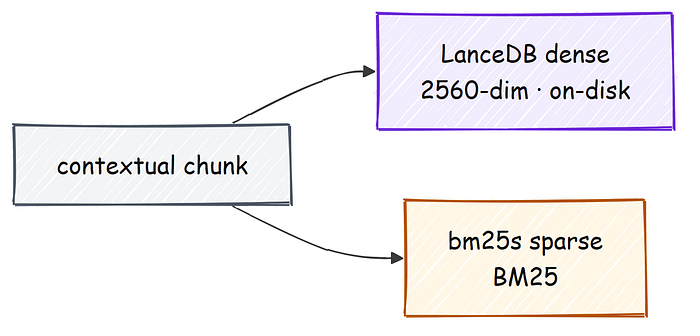
The hybrid index stores every chunk twice: a dense vector in LanceDB and a sparse BM25 posting (Created by
)
混合式索引把每個區塊存兩次:一個在 LanceDB 中的稠密向量,以及一個稀疏的 BM25 倒排項(由
製作)
We load the embedder just for indexing, embed every chunk, and free it before serving queries with a smaller online embedder. The vectors are normalized so cosine similarity is a plain dot product.
我們只為了索引而載入嵌入器,把每個區塊嵌入,然後在用一個較小的線上(online)嵌入器提供查詢服務之前把它釋放掉。向量經過正規化,所以餘弦相似度(cosine similarity)就只是一個單純的內積(dot product)。
def embed_texts(embedder, texts, is_query: bool = False) -> np.ndarray:
    kw = {"normalize_embeddings": True, "convert_to_numpy": True, "batch_size": 64}
    if is_query:                       # Qwen3-Embedding wants a query instruction prompt
        kw["prompt_name"] = "query"
    return embedder.encode(texts, **kw).astype("float32")
Loading the query embedder is the last thing to push VRAM, and the snapshot shows where we land.
載入查詢用的嵌入器是最後一件把 VRAM 往上推的事,而快照顯示我們最終落在哪裡。
That peak is about 62 GB of the 80, still inside budget, and I free the heavier offline embedder right after indexing so only the small online one stays resident for queries. I have to choose LanceDB for the dense side because it is embedded and on-disk on NVMe with no server to run, which means the same code path holds an index far larger than RAM, and that one property is what lets this design reach 10M+ vectors later without changing a line.
那個峰值大約是 80 GB 中的 62 GB,仍在預算之內,而我在索引完成後立刻釋放那個較重的離線(offline)嵌入器,好讓只有那個小小的線上嵌入器常駐以供查詢。我必須為稠密側選擇 LanceDB,因為它是嵌入式(embedded)、放在 NVMe 上的磁碟儲存、不需要跑任何伺服器,這意味著同一條程式碼路徑能容納一個遠比 RAM 大的索引,而正是這一項特性,讓這個設計稍後能在不改動一行程式碼的情況下達到超過一千萬個向量。
The dense side is a thin wrapper over it. The only subtlety is turning cosine distance back into a similarity in the zero-to-one range.
稠密側只是它的一層薄薄包裝。唯一微妙之處,是把餘弦距離(cosine distance)換算回一個落在 0 到 1 範圍內的相似度。
class LanceVectorStore:
    def search(self, qvec: np.ndarray, k: int) -> list[tuple[str, float]]:
        res = self.tbl.search(qvec).metric("cosine").limit(k).to_list()
        # cosine _distance is in [0, 2], so convert it to a similarity in [0, 1]
        return [(r["id"], 1.0 - r["_distance"] / 2.0) for r in res]
I keep a lexical bm25s index alongside the vectors because dense embeddings are exactly the thing that blurs a rare name, an id, or a number into its neighbors, and those are often the tokens a factual question turns on, so the sparse side is my insurance against a confident answer built on a near-miss passage. The sparse side stems the query the same way it stemmed the documents, then returns the top matches by BM25 score.
我在向量旁邊保留一個詞彙式(lexical)的 bm25s 索引,因為稠密嵌入正是那個會把罕見名字、id 或數字模糊成鄰近字詞的東西,而那些往往是一個事實性問題所仰賴的 token,所以稀疏側是我對「建立在差一點錯過的段落上的自信答案」的保險。稀疏側對查詢做和它對文件相同方式的詞幹處理(stem),然後依 BM25 分數回傳頂端的比對結果。
class BM25Index:
    def search(self, query: str, k: int) -> list[tuple[str, float]]:
        q = bm25s.tokenize(query, stemmer=self.stemmer)
        idx, scores = self.retriever.retrieve(q, k=min(k, len(self.ids)))
        return [(self.ids[int(i)], float(s)) for i, s in zip(idx[0], scores[0])]
The whole index for these 21,259 chunks is about 11.1 MB on disk, which is tiny, but the point is the shape, not the size. LanceDB keeps the vectors on NVMe rather than in RAM, so the same code path holds an index that is far larger than memory. That is the property we lean on at the end of the blog when we push this design to ten million vectors.
這 21,259 個區塊的整個索引在磁碟上大約 11.1 MB,非常小,但重點在於形態(shape),而不是大小。LanceDB 把向量放在 NVMe 上而非 RAM 中,因此同一條程式碼路徑能容納一個遠比記憶體大的索引。那正是我們在部落格結尾把這個設計推向一千萬個向量時所倚賴的特性。
Retrieval: Fusion and Reranking / 檢索:融合與重新排序
Reciprocal rank fusion / 倒數排名融合
We have two ranked lists now, one dense and one sparse, and we have to combine them. The trap is that their scores are not comparable, because a BM25 score and a cosine similarity live on different scales.
我們現在有兩份排名清單,一份稠密、一份稀疏,我們必須把它們合併。陷阱在於它們的分數無法相比,因為一個 BM25 分數和一個餘弦相似度活在不同的尺度上。
Reciprocal rank fusion sidesteps that completely. It ignores the scores and uses only the rank, giving each result a weight of one over k plus its rank, then sums those weights across both lists.
倒數排名融合完全繞過了這一點。它忽略分數、只用排名,給每一個結果一個「1 除以(k 加上它的排名)」的權重,然後把這些權重在兩份清單上加總起來。
Press enter or click to view image in full size
按下 Enter 或點擊以檢視完整尺寸圖片

Reciprocal rank fusion combines the dense and sparse rankings by rank, with no score normalization (Created by
)
倒數排名融合依排名把稠密與稀疏的排名合併起來,不需要任何分數正規化(由
製作)
def rrf_fuse(rankings: list[list[str]], k: int = 60) -> list[tuple[str, float]]:
    scores: dict[str, float] = {}
    for ranking in rankings:
        for rank, cid in enumerate(ranking):
            # a later rank adds less, and no score normalization is needed
            scores[cid] = scores.get(cid, 0.0) + 1.0 / (k + rank + 1)
    return sorted(scores.items(), key=lambda x: -x[1])
It is easier to see than to describe. Take two short rankings where the dense list and the sparse list disagree, and watch what fusion does.
這用看的比用講的容易懂。拿兩份稠密清單與稀疏清單意見相左的短排名,看看融合做了什麼。
#### OUTPUT ####
>>> rrf_fuse([["a", "b", "c"], ["b", "c", "a"]])
[('b', 0.03252), ('a', 0.03227), ('c', 0.03200)]
Document b wins even though neither list put it first, because it sits near the top of both. That is the whole point.
文件 b 勝出,即使兩份清單都沒把它排第一,因為它在兩份清單裡都靠近頂端。這正是重點所在。
A result two different retrievers agree on rises above a result only one of them loved. The reason we fuse at all is that the two retrievers fail in different ways.
一個兩個不同檢索器都認同的結果,會升到一個只有其中一個偏愛的結果之上。我們之所以要融合,正是因為這兩個檢索器以不同的方式失敗。
Dense search misses a rare proper noun that does not sit near anything it has seen in embedding space, and sparse search misses a paraphrase that shares no words with the query, so fusing them recovers the documents each one alone would have dropped. The retriever ties them together, embedding the query once, running both searches at the same width, and fusing the two id rankings into one.
稠密搜尋會漏掉一個罕見的專有名詞,因為它在嵌入空間裡不靠近任何它看過的東西;而稀疏搜尋會漏掉一個和查詢沒有共用任何字詞的改寫,所以融合它們就能把兩者各自單獨會丟掉的文件救回來。檢索器把它們綁在一起,把查詢嵌入一次、以相同的寬度執行兩種搜尋,並把兩份 id 排名融合成一份。
class HybridRetriever:
    def retrieve(self, query: str, k: int) -> list[RetrievedChunk]:
        qvec = embed_texts(self.embedder, [query], is_query=True)[0]
        dense = self.vec.search(qvec, k)        # dense catches paraphrase and meaning
        sparse = self.bm25.search(query, k)     # sparse catches exact names, ids, numbers
        fused = rrf_fuse([[i for i, _ in dense], [i for i, _ in sparse]], self.rrf_k)[:k]
        return [c for c in (self._mk(cid, s, "hybrid") for cid, s in fused) if c]
The fused list is our recall stage, deliberately wide at 150 candidates, because the next stage is where we trade that recall for precision.
這份融合後的清單是我們的召回階段,刻意設得很寬、有 150 個候選,因為下一個階段正是我們拿那份召回率去換取精確度(precision)的地方。
Reranking / 重新排序
Recall is cheap and precision is expensive, so we run them in that order. The reranker we loaded earlier reads the query and a candidate together and scores how well they match, which is far more accurate than the bi-encoder embeddings but far too slow to run over the whole corpus.
召回便宜、精確度昂貴,所以我們照這個順序來跑。我們稍早載入的重新排序器把查詢與一個候選一起讀進來,並為它們的匹配程度評分,這遠比雙編碼器(bi-encoder)嵌入精準,卻慢到不可能在整個語料庫上跑。
Running it over only the 150 fused candidates is the sweet spot. Running the expensive model on 150 candidates instead of the whole corpus is also a scaling decision, because that cost is fixed at 150 pairs whether the index holds twenty thousand chunks or ten million.
只在那 150 個融合後的候選上跑它,正是甜蜜點。在 150 個候選、而非整個語料庫上跑這個昂貴的模型,也是一個關於擴展的決策,因為無論索引裝的是兩萬個區塊還是一千萬個,這個成本都固定在 150 對。
A thin stage wraps the model, scores every candidate, and keeps the top twenty.
一個薄薄的階段包裝這個模型,為每個候選評分,並保留前二十名。
Press enter or click to view image in full size
按下 Enter 或點擊以檢視完整尺寸圖片

Reranking takes the 150 fused candidates and keeps the 20 best by the reranker score (Created by
)
重新排序拿那 150 個融合後的候選,並依重新排序器的分數留下最好的 20 個(由
製作)
class RerankerStage:
    def rerank(self, query, cands, top_n):
        scores = self.reranker.score(query, [c.text for c in cands])
        ranked = sorted(zip(cands, scores), key=lambda x: -x[1])[:top_n]
        out = []
        for c, s in ranked:
            c.score, c.source = float(s), "reranked"
            out.append(c)
        return out
We can prove the lift by measuring passage recall against the HotpotQA gold titles, dense alone, then hybrid, then reranked, on our running example.
我們可以在我們一路追蹤的範例上,對照 HotpotQA 的黃金標題來衡量段落召回率——先是單獨的稠密、再是混合、再是重新排序後——以此證明這份提升。
#### OUTPUT ###
Q: Were Scott Derrickson and Ed Wood of the same nationality?
 gold titles: ['Scott Derrickson', 'Ed Wood']
 recall@20:  dense=1.00  hybrid=1.00  reranked=1.00
 top-3 reranked:
   [a9ec406223bd] (0.999) Scott Derrickson
   [2d2201c92ac5] (0.996) Ed Wood
   [b7dbb0e190b4] (0.796) Ed Wood (film)
Both gold passages land in the top three with reranker scores of 0.999 and 0.996, while the less relevant film article sits lower at 0.796. Across the full evaluation this retrieval stack reaches 0.97 context recall, which means the evidence is almost always there when the question is answerable.
兩段黃金段落都落在前三名,重新排序器分數為 0.999 與 0.996,而較不相關的電影條目則以 0.796 落在較低的位置。在整個評估中,這套檢索堆疊達到 0.97 的上下文召回率(context recall),這意味著當問題可回答時,證據幾乎總是在那裡。
Retrieval is solved. Everything after this is about not abusing it.
檢索問題解決了。這之後的一切,都是關於不要濫用它。
Routing and Decomposition / 路由與分解
Not every query deserves the full pipeline. A greeting needs no retrieval, a simple lookup needs one hop, and a comparison needs several. So the first thing the agent does is route the question into one of three labels, which lets us spend compute only where it helps.
並不是每個查詢都配得上整套流程。一句問候不需要檢索,一次簡單的查找需要一跳,一個比較則需要好幾跳。所以代理做的第一件事,就是把問題路由(route)成三個標籤之一,這讓我們只在有幫助的地方花費算力。
Press enter or click to view image in full size
按下 Enter 或點擊以檢視完整尺寸圖片
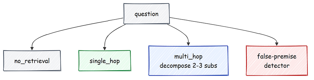
The router sends each question down a no_retrieval, single_hop, or multi_hop path, with a separate false-premise check (Created by
)
路由器把每個問題送往 no_retrieval、single_hop 或 multi_hop 的路徑,並附帶一個獨立的假前提檢查(由
製作)
ROUTER_PROMPT = (
    "Classify the question into exactly one label:\n"
    "- no_retrieval: greetings/opinions or questions no document corpus could answer\n"
    "- single_hop: answerable by finding one fact\n"
    "- multi_hop: needs combining facts from multiple documents\n"
    "Question: {q}\nReply with only the label."
)

class QueryRouter:
    LABELS = {"no_retrieval", "single_hop", "multi_hop"}

    def route(self, query: str) -> str:
        out = self.llm.chat("You are a precise query classifier.",
                            ROUTER_PROMPT.format(q=query), max_tokens=8).strip().lower()
        for lbl in self.LABELS:
            if lbl in out:
                return lbl
        return "single_hop"                 # a safe default if the model is chatty
The decomposer and the false-premise check are just as small. The decomposer asks for two or three self-contained sub-questions, and the detector asks a blunt yes-or-no question about whether the query assumes something that may not be true.
分解器(decomposer)與假前提檢查同樣小巧。分解器要求生成兩到三個自成一體(self-contained)的子問題,而偵測器則直白地問一個是非題:這個查詢是否假設了某件可能不為真的事。
DECOMPOSE_PROMPT = (
    "Break this multi-hop question into 2-3 ordered, self-contained sub-questions, "
    "one per line, no numbering. If it is already simple, return it unchanged.\nQuestion: {q}"
)

def detect_false_premise(query: str, llm: LocalLLM) -> bool:
    out = llm.chat("You detect false presuppositions.",
                   FALSE_PREMISE_PROMPT.format(q=query), max_tokens=4)
    return out.strip().lower().startswith("y")
#### OUTPUT ####
route('Were Scott Derrickson and Ed Wood of the same nationality?...') -> single_hop
decompose ->
   • What is the nationality of Scott Derrickson?
   • What is the nationality of Ed Wood?
The same router on two other kinds of question shows the other branches.
同一個路由器套用在另外兩種問題上,展示了其他分支。
#### OUTPUT ####
route('What is the best programming language?') -> no_retrieval
route('Who directed Ed Wood, and what is that director also known for?') -> multi_hop
An opinion gets no_retrieval, which is itself an abstention path, because the system declines rather than search for an answer no document holds. A real two-fact question gets multi_hop, which is what later sends the agent into its corrective loop.
一個意見得到 no_retrieval,這本身就是一條棄答路徑,因為系統選擇拒絕,而不是去搜尋一個沒有任何文件握有的答案。一個真正的雙事實問題得到 multi_hop,那正是稍後把代理送進它修正迴圈的原因。
The router calls our running example single-hop because the reranked passages already answer it directly, and the decomposer still shows how it would break the comparison into two clean lookups if the first pass came back thin. Routing is cheap, a single short classification call, and it earns its place by keeping the expensive retrieval and verification work off the questions that do not need it, which also matters at scale because every retrieval I skip is latency I do not spend.
路由器把我們一路追蹤的範例判定為 single_hop,因為重新排序後的段落已經直接回答了它,而分解器仍然展示了:若第一輪回來的內容很薄弱,它會如何把這個比較拆成兩次乾淨的查找。路由很便宜,只是一次短短的分類呼叫,而它靠著讓昂貴的檢索與驗證工作遠離那些不需要它的問題來贏得它的一席之地,這在規模下也很重要,因為我每跳過的一次檢索,都是我沒有花掉的延遲。
Cited Generation / 帶引用的生成
This is the first hallucination firewall. The system prompt forbids outside knowledge, requires an inline citation for every sentence, and gives the model an explicit token to emit when the context does not contain the answer. Telling the model to cite is not enough on its own, so we also validate the citations and drop any the model invented.
這是第一道幻覺防火牆。系統提示禁止使用外部知識、要求每一句都有行內引用,並給模型一個明確的 token,好讓它在上下文不含答案時輸出。光是叫模型引用還不夠,所以我們也會驗證這些引用,並丟棄任何模型憑空捏造的。
Press enter or click to view image in full size
按下 Enter 或點擊以檢視完整尺寸圖片

Cited generation: answer only from context with a citation per sentence, abstain otherwise, and strip any invalid citation (Created by
)
帶引用的生成:只根據上下文作答、每句附一個引用,否則棄答,並剝除任何無效的引用(由
製作)
ABSTAIN_TOKEN = "INSUFFICIENT_EVIDENCE"
GENERATION_SYSTEM_PROMPT = (
    "You answer strictly from the numbered context passages. Rules:\n"
    "1. Use ONLY facts in the passages, never outside knowledge.\n"
    f"2. If the passages do not contain the answer, reply with exactly: {ABSTAIN_TOKEN}\n"
    "3. Every sentence MUST end with a citation to the passage id(s) it uses, like [abc123def456].\n"
    "4. Be concise and factual."
)
After generation we parse the citation markers and keep only the ones that match a real chunk id, so a fabricated citation can never survive to the user.
生成之後,我們解析引用標記,只保留那些對應到真實區塊 id 的,這樣一個被捏造的引用就永遠不可能存活到使用者面前。
def parse_citations(text: str, valid_ids: set[str]) -> tuple[list[str], str]:
    found = _CITE_RE.findall(text)
    valid = [c for c in dict.fromkeys(found) if c in valid_ids]
    invalid = [c for c in dict.fromkeys(found) if c not in valid_ids]
    cleaned = text
    for bad in invalid:                       # strip any citation the model invented
        cleaned = cleaned.replace(f"[{bad}]", "")
    return valid, cleaned
Run it on a sentence that cites one real passage and one the model invented, and the fake citation simply disappears.
把它套用在一句引用了一段真實段落、以及一段模型捏造段落的句子上,那個假引用就這麼消失了。
#### OUTPUT ####
>>> text = "Paris is the capital of France [a1b2c3d4e5f6]. The Louvre opened in 1793 [deadbeef0000]."
>>> parse_citations(text, valid_ids={"a1b2c3d4e5f6"})
(['a1b2c3d4e5f6'], 'Paris is the capital of France [a1b2c3d4e5f6]. The Louvre opened in 1793 .')
The valid id stays and the invented [deadbeef0000] is stripped, so only a real citation reaches the next stage. This matters because the most dangerous hallucination is a confident sentence wearing a citation it did not earn, and here that citation is gone before anyone sees it. The generator formats the retrieved passages with their ids, calls the model once, and either returns the abstain signal or a parsed, citation-checked answer.
有效的 id 留下,而捏造的 [deadbeef0000] 被剝除,所以只有真實的引用能進入下一個階段。這很重要,因為最危險的幻覺,是一句自信的句子披著它並未贏得的引用,而在這裡,那個引用在任何人看到它之前就已經不見了。生成器把檢索到的段落連同它們的 id 一起格式化,呼叫模型一次,然後不是回傳棄答訊號、就是回傳一個經過解析、引用檢查過的答案。
class CitedGenerator:
    def generate(self, question, chunks) -> CitedAnswer:
        user = f"Context passages:\n{format_context(chunks)}\n\nQuestion: {question}\n\nAnswer:"
        raw = self.llm.chat(GENERATION_SYSTEM_PROMPT, user, max_tokens=400).strip()
        if ABSTAIN_TOKEN in raw:                          # the model chose to abstain
            return CitedAnswer(text="", cited_ids=[], abstained=True, raw=raw)
        cited, cleaned = parse_citations(raw, {c.id for c in chunks})
        return CitedAnswer(text=cleaned.strip(), cited_ids=cited, abstained=False, raw=raw)
#### OUTPUT ####
Q: Were Scott Derrickson and Ed Wood of the same nationality?
abstained=False  citations=['a9ec406223bd', '2d2201c92ac5']
A: Yes, Scott Derrickson and Ed Wood were of the same nationality; both were American. [a9ec406223bd] [2d2201c92ac5]
The answer cites the two passages we retrieved, and both ids are real, so nothing gets stripped. At this point we have a fluent, cited answer, but a citation only proves the model pointed at a passage, not that the passage actually supports what it said.
答案引用了我們檢索到的兩段段落,而兩個 id 都是真的,所以沒有任何東西被剝除。到此為止,我們有了一個流暢、帶引用的答案,但一個引用只證明了模型指向了某段段落,並不能證明那段段落確實支持它所說的話。
A model can cite a real passage and still misread it, so a citation is necessary but not sufficient. That gap is what the next firewall closes.
一個模型可以引用一段真實段落,卻仍然誤讀它,所以引用是必要的、但並不充分。而那道缺口,正是下一道防火牆所要封閉的。
The Verification Gate / 驗證關卡
This is the decisive firewall. We split the drafted answer into atomic claims, then check each claim against its cited context with the faithfulness judge we loaded earlier. A claim that scores below the threshold is unsupported, and if any claim fails, the whole answer is downgraded to an abstention.
這是決定性的防火牆。我們把草擬的答案拆成原子級主張,接著用我們稍早載入的忠實度評判者,把每個主張與它所引用的上下文逐一比對。一個分數低於門檻的主張是未獲支持的,而只要任何一個主張失敗,整個答案就被降級為棄答。
Press enter or click to view image in full size
按下 Enter 或點擊以檢視完整尺寸圖片

The verification gate splits the answer into atomic claims, scores each against the cited context, and abstains if any falls below tau (Created by
)
驗證關卡把答案拆成原子級主張,將每一個對照所引用的上下文評分,並在任何一個落到 tau(門檻)以下時棄答(由
製作)
The claim extractor splits the answer into atomic, independently checkable statements, dropping the citation markers first so the claims are clean text.
主張抽取器(claim extractor)把答案拆成原子級、可獨立檢查的陳述,並先丟掉引用標記,讓這些主張是乾淨的文字。
class ClaimExtractor:
    def extract(self, answer: str) -> list[str]:
        clean = _CITE_RE.sub("", answer).strip()          # remove [id] markers first
        out = self.llm.chat("You extract atomic factual claims.",
                            CLAIM_DECOMP_PROMPT.format(a=clean), max_tokens=300)
        claims = [re.sub(r"^\s*\d+[.)]\s*", "", ln).strip(" -\t")
                  for ln in out.splitlines() if ln.strip()]
        return [c for c in claims if len(c) > 3]
The gate extracts the claims, scores each against the cited passages, and passes only if every claim clears the threshold.
關卡抽取這些主張,把每一個對照所引用的段落評分,並且只有在每一個主張都通過門檻時才放行。
class VerificationGate:
    def check(self, cited: CitedAnswer, chunks: list[RetrievedChunk]) -> GateResult:
        claims = self.extractor.extract(cited.text)            # split into atomic claims
        used = [c for c in chunks if c.id in set(cited.cited_ids)] or chunks
        context = "\n\n".join(c.text for c in used)
        verdicts = []
        for cl in claims:
            s = self.verifier.support(cl, context)
            verdicts.append(ClaimVerdict(cl, s["score"], s["score"] >= self.tau,
                                         s["nli"], s["minicheck"]))
        min_support = min((v.score for v in verdicts), default=0.0)
        passed = len(verdicts) > 0 and all(v.supported for v in verdicts)
        return GateResult(passed, verdicts, min_support, len(verdicts))
#### OUTPUT ####
claims=3  passed=True  min_support=1.00
   [OK 1.00] Scott Derrickson is American.
   [OK 1.00] Ed Wood is American.
   [OK 1.00] Scott Derrickson and Ed Wood share the same nationality.
The one-sentence answer breaks into three checkable claims, and each one scores a full 1.00 against the cited passages, so the gate passes with a minimum support of 1.00. Checking at the claim level instead of the whole answer is what makes this strict.
這一句話的答案拆成了三個可檢查的主張,而每一個對照所引用的段落都拿到滿分 1.00,所以關卡以 1.00 的最低支持度放行。在主張層級、而非整個答案層級進行檢查,正是讓這件事變得嚴格的原因。
A long answer can be eighty percent grounded and still smuggle in one invented fact, and an answer-level score would wave it through, while a claim-level gate isolates that one sentence and fails on it. The key design choice is that the gate reports the weakest claim, not the average, because an answer is only as trustworthy as its least supported sentence.
一個長答案可以有百分之八十有所依據,卻仍然夾帶進一個捏造的事實,而答案層級的分數會讓它矇混過關,而主張層級的關卡則會把那一句隔離出來、並因它而不通過。關鍵的設計選擇是:關卡回報的是最弱的主張,而非平均,因為一個答案的可信度,只取決於它獲得支持最少的那一句。
That weakest-claim rule is best seen when it fires. Here is the same gate on a draft for one of the false-premise questions, where the model tried to oblige.
最弱主張這條規則,在它觸發時最看得清楚。這裡是同一個關卡,套用在一個假前提問題的草稿上——模型試圖去迎合它。
#### OUTPUT ####
claims=2  passed=False  min_support=0.20
   [OK 0.95] Marie Curie was a physicist.
   [XX 0.20] Marie Curie traveled to the Moon.
The first claim is well supported, but the second scores 0.20, far below the 0.3 threshold, because no passage says any such thing. One failing claim flips passed to False, the whole answer is thrown out, and the question becomes an abstention instead of a confident false statement. This is the exact moment a hallucination is caught and turned into a safe refusal.
第一個主張獲得良好的支持,但第二個只拿到 0.20,遠低於 0.3 的門檻,因為沒有任何段落說過這種事。一個失敗的主張就把 passed 翻轉成 False,整個答案被丟棄,而這個問題就變成一次棄答,而不是一句自信的錯誤陳述。這正是一個幻覺被逮到、並被轉化為一次安全拒絕的那一刻。
For a borderline answer we do not just throw it away. A chain-of-verification pass gives it one chance to repair itself, rewriting any sentence the context does not support and keeping the citations, and then the gate runs again on the revised text.
對於一個模稜兩可的答案,我們並不只是把它丟掉。一次驗證鏈(chain-of-verification)的處理給它一個自我修復的機會,改寫任何上下文不支持的句子並保留引用,然後關卡再對修訂後的文字重跑一次。
COVE_PROMPT = (
    "Revise the answer so EVERY sentence is directly supported by the context. "
    "Remove or soften any claim not supported. Keep citations [id].\n\n"
    "Context:\n{ctx}\n\nAnswer:\n{ans}\n\nRevised answer:"
)

def cove_revise(answer: str, chunks, llm: LocalLLM) -> str:
    ctx = format_context(chunks)
    return llm.chat("You make answers strictly faithful to context.",
                    COVE_PROMPT.format(ctx=ctx, ans=answer), max_tokens=400).strip()
Knowing When to Abstain / 懂得何時該棄答
Abstention is a correct answer, not a failure, so we make it a first-class outcome. This is the move that makes near-zero hallucination possible at all.
棄答是一個正確的答案,而不是一次失敗,所以我們把它當作一種一等(first-class)的結果。這正是讓近乎零幻覺得以成為可能的那一步。
I cannot stop the model from being wrong on a question with no answer in the corpus, but I can make the system refuse that question, which turns an unbounded failure, a confident lie, into a bounded one, a visible abstention I can measure and tune. The policy folds the signals into one decision.
對於一個在語料庫裡沒有答案的問題,我無法阻止模型出錯,但我可以讓系統拒絕那個問題,這把一個無界(unbounded)的失敗——一個自信的謊言——轉化成一個有界(bounded)的失敗——一次我能衡量並調整的、可見的棄答。這個策略(policy)把各種訊號匯整成一個決策。
If the router said no retrieval, or the model emitted the abstain token, or the verification gate failed, we abstain, and otherwise we answer with the verified text.
如果路由器說了不檢索、或模型輸出了棄答 token、或驗證關卡失敗,我們就棄答;否則我們就用經過驗證的文字來作答。
Press enter or click to view image in full size
按下 Enter 或點擊以檢視完整尺寸圖片
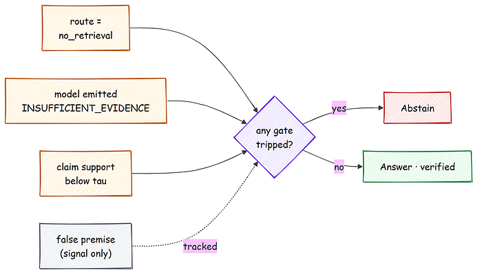
The abstention policy: three hard gates send a question to abstain, the verified path sends it to answer, and false premise is a tracked signal (Created by
)
棄答策略:三道硬性關卡把一個問題送去棄答,經過驗證的路徑把它送去作答,而假前提是一個被追蹤的訊號(由
製作)
Every outcome is one strict, auditable record, so evaluation can parse answered against abstained without any guesswork.
每一個結果都是一筆嚴格、可稽核(auditable)的紀錄,如此一來評估就能在毫無猜測的情況下把「已作答」與「已棄答」解析開來。
@dataclass
class FinalAnswer:
    status: str               # "answered" or "abstained"
    answer: str
    citations: list[str]
    min_support: float
    reason: str               # which gate fired, or "verified"
class AbstentionPolicy:
    def decide(self, route, false_premise, cited, gate) -> FinalAnswer:
        if route == "no_retrieval":
            return self._abstain("routed_no_retrieval", gate)
        if cited.abstained:
            return self._abstain("model_abstained", gate)
        if gate is None or not gate.passed or gate.min_support < self.tau:
            return self._abstain("unsupported_claims", gate)
        return FinalAnswer("answered", cited.text, cited.cited_ids,
                           gate.min_support, "verified", {})
#### OUTPUT ####
AbstentionPolicy ready; reasons = {routed_no_retrieval, false_premise, model_abstained, unsupported_claims, verified}
There is one subtlety worth calling out. The false-premise flag is recorded as a signal, but it is not a hard gate, because a small yes-or-no detector is too noisy to trust on its own.
有一個微妙之處值得點出。假前提的旗標(flag)被記錄為一個訊號,但它並不是一道硬性關卡,因為一個小型的是非偵測器本身雜訊太多、無法單獨信任。
We let the evidence path of grading plus claim verification make the real decision, which catches false-premise questions anyway when no passage supports them. When the system does abstain, it returns a plain message, “I do not have enough supporting evidence in the available sources to answer this confidently,” instead of a guess.
我們讓評分加上主張驗證的證據路徑來做出真正的決定,反正當沒有任何段落支持時,這條路徑也會逮到假前提問題。當系統確實棄答時,它回傳一則樸素的訊息——「我在可得的來源中沒有足夠的支持證據,無法有信心地回答這個問題」——而不是一個猜測。
The Agent / 代理
We have now built every component, so the last step is to wire them into a graph that corrects itself, because the single biggest cause of hallucination is generating from bad context. The loop is built with LangGraph, which I choose because the control flow is genuinely a graph and not a straight line, route can skip retrieval, grade can loop back through refine, and verify can downgrade an answer to an abstention, so I would rather declare those edges than bury them in nested conditionals.
我們現在已經建好了每一個元件,所以最後一步是把它們接成一張會自我修正的圖(graph),因為造成幻覺的最大單一原因,就是從糟糕的上下文中生成。這個迴圈是用 LangGraph 建的,我之所以選它,是因為控制流程真的是一張圖、而不是一條直線——route 可以跳過檢索、grade 可以透過 refine 迴圈折返、而 verify 可以把一個答案降級為棄答,所以我寧可明確宣告那些邊(edge),也不願把它們埋進層層巢狀的條件判斷裡。
We route, retrieve, then grade the evidence. If the evidence is strong we generate, if it is weak we refine the query and retrieve again up to a hop cap, and if it is hopeless we abstain without ever generating.
我們先路由、檢索,然後為證據評分(grade)。如果證據強,我們就生成;如果它薄弱,我們就精煉(refine)查詢並在一個跳躍上限(hop cap)之內重新檢索;如果它毫無希望,我們就棄答,完全不進行生成。
Press enter or click to view image in full size
按下 Enter 或點擊以檢視完整尺寸圖片

The CRAG loop grades its own evidence, refines and re-retrieves when it is weak, and only generates when the evidence is strong enough (Created by
)
CRAG 迴圈為它自己的證據評分,在證據薄弱時精煉並重新檢索,並且只在證據夠強時才生成(由
製作)
The agent passes one state object between nodes, a typed dictionary that accumulates the route, the evidence, the grade, the draft, the gate result, and a running latency tally.
代理在各節點(node)之間傳遞一個狀態物件,一個帶型別(typed)的字典,累積路由、證據、評分、草稿、關卡結果,以及一份持續累加的延遲統計。
class AgentState(TypedDict, total=False):
    question: str
    route: str
    query: str
    evidence: list
    grade: float
    draft: Any
    gate: Any
    final: Any
    hops: int
    latencies: dict
Each node does one job. The grader scores how well the current passages answer the question, and the refine node is the corrective step, it bumps the hop counter, decomposes the question, and widens the query before we retrieve again.
每個節點做一件工作。評分者為當前段落回答問題的程度打分,而 refine 節點是那個修正步驟,它把跳躍計數器加一、分解問題,並在我們再次檢索之前拓寬查詢。
def grade_evidence(query: str, chunks, llm: LocalLLM) -> float:
    ctx = "\n".join(f"- {c.text[:200]}" for c in chunks[:8])
    out = llm.chat("You grade retrieval sufficiency.",
                   GRADE_PROMPT.format(q=query, ctx=ctx), max_tokens=8)
    m = re.search(r"[01](?:\.\d+)?", out)
    return float(m.group()) if m else 0.5

def n_refine(state: AgentState) -> AgentState:
    state["hops"] = state.get("hops", 0) + 1
    subs = decomposer.decompose(state["question"])
    state["query"] = " ".join(subs)          # broaden the query with the sub-questions
    return state
A small routing function turns the grade into the next move, and the graph wires the nodes together with the refine step looping back to retrieve.
一個小小的路由函式把評分轉成下一步的動作,而這張圖把各節點接在一起,讓 refine 步驟折返回 retrieve。
def _after_grade(state: AgentState) -> str:
    g = state.get("grade", 0.0)
    if g >= CRAG_OK:                       # 0.7+, the evidence is strong, answer it
        return "generate"
    if g < CRAG_BAD or state.get("hops", 0) >= MAX_HOPS:
        return "generate" if g >= CRAG_BAD else "finalize"   # too weak, abstain
    return "refine"                        # borderline, refine the query and retry


def build_agent_graph():
    g = StateGraph(AgentState)
    for name, fn in [("route", n_route), ("retrieve", n_retrieve), ("grade", n_grade),
                     ("refine", n_refine), ("generate", n_generate),
                     ("verify", n_verify), ("finalize", n_finalize)]:
        g.add_node(name, fn)
    g.set_entry_point("route")
    g.add_conditional_edges("grade", _after_grade,
                            {"generate": "generate", "refine": "refine", "finalize": "finalize"})
    g.add_edge("refine", "retrieve")       # the corrective loop
    g.add_edge("generate", "verify")
    g.add_edge("verify", "finalize")
    return g.compile()
Running the full agent over our running example shows every stage and its timing.
在我們一路追蹤的範例上執行完整的代理,會顯示出每一個階段及其計時。
#### OUTPUT ####
Q: Were Scott Derrickson and Ed Wood of the same nationality?
route=single_hop hops=0 grade=1.00 status=answered reason=verified
A: Yes, Scott Derrickson and Ed Wood were of the same nationality; both were American.
latencies(s): {'route': 0.16, 'retrieve': 2.4, 'grade': 0.13, 'generate': 0.94, 'verify': 0.97, 'total': 4.6}
The grade comes back at 1.00, so the agent goes straight to generation, and the final status is answered with reason verified, which means it passed every gate we built. The hop counter stays at zero here, but on a thin retrieval it would climb to three before giving up. The bounded loop is what keeps latency in budget while still allowing a second and third try.
評分回來是 1.00,所以代理直接前往生成,而最終狀態是 answered、理由是 verified,這意味著它通過了我們所建的每一道關卡。跳躍計數器在這裡維持為零,但在一次薄弱的檢索上,它會爬到三次才放棄。這個有界的迴圈,正是讓延遲維持在預算內、同時仍允許第二次和第三次嘗試的關鍵。
The contrast is the whole design in two lines. Send the agent a question with no answer in the corpus, and the same graph reaches the opposite, correct conclusion.
這份對比用兩行就概括了整個設計。給代理一個在語料庫裡沒有答案的問題,同一張圖會抵達相反、且正確的結論。
#### OUTPUT ####
Q: Which programming language did Isaac Newton invent in 1700?
route=single_hop hops=0 grade=0.15 status=abstained reason=unsupported_claims
A: I do not have enough supporting evidence in the available sources to answer this confidently.
latencies(s): {'route': 0.17, 'retrieve': 2.9, 'grade': 0.14, 'total': 3.3}
Retrieval finds nothing about Newton inventing a language, so the grade comes back at 0.15, below the crag_bad floor of 0.4, and the agent finalizes straight to an abstention without ever generating. That early exit is also why the abstain path is faster, 3.3 seconds here against 4.6 for the answered case, because the system spends nothing on generation or verification once it knows the evidence is not there. This is what the 98 out of 100 abstentions on the unanswerable set look like, one question at a time.
檢索找不到任何關於牛頓發明語言的東西,所以評分回來是 0.15,低於 crag_bad 的下限 0.4,於是代理直接定案(finalize)成棄答,完全不進行生成。那次提前退出也是棄答路徑之所以較快的原因——這裡是 3.3 秒,相對於已作答情況的 4.6 秒——因為一旦系統知道證據不在那裡,它就不會在生成或驗證上花費任何東西。這就是不可回答集上 100 題中 98 次棄答的樣子,一次一題。
Does It Work? / 它真的有效嗎?
The golden set / 黃金測試集
To measure any of this we need a test set with two strata. The answerable stratum comes from HotpotQA, and the unanswerable stratum comes from SQuAD v2 impossible questions plus a handful of hand-built false-premise questions.
要衡量這一切,我們需要一個具有兩個層別的測試集。可回答層別來自 HotpotQA,而不可回答層別則來自 SQuAD v2 的無解問題外加少量手工打造的假前提問題。
The unanswerable half is the important one, because it is where a normal RAG system quietly bluffs. Everything we built, the citation rule, the claim gate, the abstention policy, exists to keep that half quiet, so this is the stratum that actually scores the near-zero hallucination claim, while the answerable half scores whether retrieval did its job.
不可回答的那一半才是重要的,因為那正是一套普通的 RAG 系統會悄悄唬弄的地方。我們所建的一切——引用規則、主張關卡、棄答策略——存在的目的就是讓那一半保持沉默,所以這是實際上為近乎零幻覺這項主張評分的層別,而可回答的那一半則評估檢索是否做好了它的工作。
Press enter or click to view image in full size
按下 Enter 或點擊以檢視完整尺寸圖片
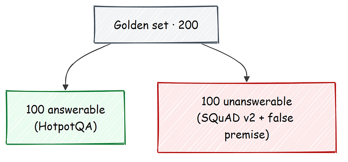
The golden set is 100 answerable questions and 100 unanswerable ones, including hand-built false-premise questions (Created by
)
黃金測試集是 100 個可回答問題與 100 個不可回答問題,包含手工打造的假前提問題(由
製作)
def build_false_premise_set() -> list[EvalItem]:
    qs = [
        "In what year did Albert Einstein win his second Nobel Prize in Physics?",
        "What was the name of the spaceship Marie Curie flew to the Moon?",
        "How many gold medals did William Shakespeare win at the Olympics?",
        "Which programming language did Isaac Newton invent in 1700?",
    ]
    return [EvalItem(f"fp_{i}", q, "", [], False, "false_premise") for i, q in enumerate(qs)]
We end up with a balanced 200 question set, half answerable and half not. The false-premise questions are deliberately absurd, like asking which language Newton invented in 1700, because a system that answers those is a system that will invent facts for any confident-sounding question.
我們最終得到一個平衡的 200 題測試集,一半可回答、一半不可回答。這些假前提問題刻意設計得很荒謬,像是問牛頓在 1700 年發明了哪種語言,因為一套會回答那些問題的系統,就是一套會為任何聽起來很有把握的問題捏造事實的系統。
Balancing the two halves matters, because a set that is mostly answerable would let a system score well while still bluffing on the hard cases. Half of this set exists purely to measure restraint.
平衡這兩半很重要,因為一個大多可回答的測試集,會讓一套系統得到不錯的分數、卻仍在困難的案例上唬弄。這個測試集有一半純粹是為了衡量克制(restraint)而存在。
Hallucinations live in one cell / 幻覺只住在一個格子裡
Now we run the agent over all 200 questions and score the result as a two-by-two table. The rows are answerable or unanswerable, the columns are answered or abstained, and the one dangerous cell is unanswerable and answered, because that is a hallucination by definition.
現在我們在全部 200 個問題上執行代理,並把結果評分成一張二乘二的表。列(row)是可回答或不可回答,欄(column)是已作答或已棄答,而那唯一危險的格子是「不可回答且已作答」,因為按定義那就是一次幻覺。
def confusion_2x2(results, items) -> np.ndarray:
    cm = np.zeros((2, 2), dtype=int)   # rows: answerable/unanswerable, cols: answered/abstained
    for r, it in zip(results, items):
        i = 0 if it.answerable else 1
        j = 0 if r.final.status == "answered" else 1
        cm[i, j] += 1
    return cm
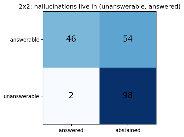
The 2x2 confusion matrix, where hallucinations are the two cases in the unanswerable and answered cell (Created by
)
二乘二的混淆矩陣(confusion matrix),其中幻覺就是「不可回答且已作答」格子裡的那兩個案例(由
製作)
#### OUTPUT ####
confusion (rows ans/unans, cols answered/abstained):
 [[46 54]
 [ 2 98]]
hallucinations (unanswerable answered): 2 / 100 unanswerable
Read the bottom row, because it is the whole point. Of the 100 unanswerable questions, the system abstained on 98 and only answered 2, which is a 2 percent hallucination rate on the questions designed to trap it.
讀最下面那一列,因為那正是全部的重點。在 100 個不可回答的問題中,系統對其中 98 個棄答、只回答了 2 個,這在那些被設計來陷害它的問題上是 2% 的幻覺率。
A plain RAG system with no verification gate would light up that cell instead, because nothing would stop it from answering a question the corpus cannot support. The top row of the matrix is what this safety costs us, and we look at it next.
一套沒有驗證關卡的普通 RAG 系統則會把那個格子點亮,因為沒有任何東西能阻止它回答一個語料庫無法支持的問題。矩陣的頂端那一列,是這份安全所付出的代價,我們接下來就來看它。
The price of safety / 安全的代價
The two-by-two used one fixed threshold, but the threshold is a dial. Turn it up and the system abstains more, which lowers hallucination but also lowers coverage. To choose it deliberately we sweep the threshold and draw a risk-coverage curve, then pick the point that keeps hallucination under a budget while answering as much as possible.
那張二乘二表用的是單一個固定的門檻,但門檻是一個旋鈕。把它調高,系統就棄答得更多,這會降低幻覺、但也降低了覆蓋率(coverage)。為了刻意地選擇它,我們掃過(sweep)門檻並畫出一條風險-覆蓋率曲線(risk-coverage curve),然後挑一個能把幻覺維持在預算之下、同時盡可能多回答的點。
def pick_tau(df, max_halluc: float = 0.05) -> float:
    # among thresholds that keep hallucination under the budget, take the most coverage
    ok = df[df["hallucination_rate"] <= max_halluc]
    return float(ok.sort_values("coverage", ascending=False).iloc[0]["tau"]) if len(ok) else 1.0
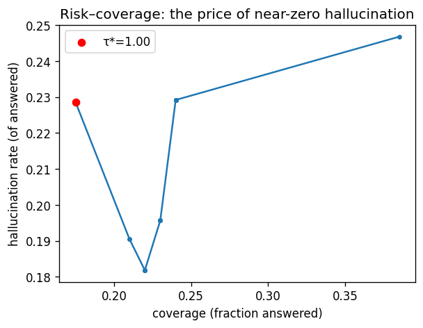
The risk-coverage curve, with the chosen operating point that holds hallucination under the budget (Created by
)
風險-覆蓋率曲線,以及那個把幻覺維持在預算之下的所選運作點(operating point)(由
製作)
#### OUTPUT ####
chosen τ* (halluc<=5%): 1.0
metrics: {
  "faithfulness": 0.908,
  "answer_relevancy": 0.817,
  "context_recall@k": 0.97,
  "answerable_accuracy": 0.58
}
On answered questions we get 0.908 faithfulness and 0.97 context recall, which says the evidence is there and the answers stay grounded in it. The price is the top row of the matrix.
在已作答的問題上,我們得到 0.908 的忠實度與 0.97 的上下文召回率,這說明證據就在那裡、而答案也維持依據著它。代價則是矩陣的頂端那一列。
We answer 46 of the 100 answerable questions and abstain on the rest, a coverage of 0.46. That is the deliberate trade.
我們回答了 100 個可回答問題中的 46 個、對其餘的棄答,覆蓋率為 0.46。那是刻意的取捨。
We would rather stay silent on a question we could have answered than risk a confident wrong answer. Where exactly you sit on this curve is a product decision and not a model one, and it can be set per corpus depending on how expensive a wrong answer is in that domain.
我們寧可在一個原本可以回答的問題上保持沉默,也不願冒著給出一個自信的錯誤答案的風險。你究竟坐在這條曲線的哪個位置,是一個產品決策、而非模型決策,而且它可以依語料庫、依那個領域裡一個錯誤答案有多昂貴來設定。
Is the judge any good? / 評判者夠好嗎?
There is a hole to close. The whole gate leans on the verifier, so an unverified verifier just moves the hallucination from the answer into the scorecard. We test the verifier on its own against HaluBench, a set of human-labeled faithful and hallucinated answers, and report the area under the ROC curve.
有一個漏洞要補上。整道關卡都倚賴驗證器,所以一個未經驗證的驗證器,只不過是把幻覺從答案裡搬進了計分卡(scorecard)。我們把驗證器單獨拿去對照 HaluBench 測試——那是一組由人類標註的忠實與幻覺答案——並回報 ROC 曲線下的面積(area under the ROC curve)。
def eval_verifier(verifier, n: int = 300) -> dict:
    hb = load_halubench().shuffle(seed=SEED).select(range(n))
    scores, labels = [], []
    for ex in hb:
        scores.append(verifier.nli_score(ex["answer"], ex["passage"]))  # the judge's support score
        labels.append(1 if str(ex["label"]).upper().startswith("PASS") else 0)
    from sklearn.metrics import roc_auc_score
    return {"auroc": round(float(roc_auc_score(labels, scores)), 3), "n": len(labels)}

The verifier ROC curve on HaluBench, with an area under the curve of 0.702 (Created by
)
驗證器在 HaluBench 上的 ROC 曲線,曲線下面積為 0.702(由
製作)
The verifier scores an AUROC of 0.702 over 300 items, which is clearly better than chance but a long way from perfect. I want to be plain about that, because it is the real ceiling on the whole gate.
驗證器在 300 個項目上拿到 0.702 的 AUROC,明顯優於隨機猜測、但離完美還很遠。我想對此坦白,因為它是整道關卡的真正天花板。
A stronger verifier is the single change that would push the numbers above further, and the architecture is built so we can drop one in without touching the rest. The gate does not need a perfect verifier to help, it needs one that ranks supported claims above unsupported ones often enough to move the operating point, and 0.702 clears that bar while leaving plenty of room to grow.
一個更強的驗證器,是那個能把上面的數字推得更遠的單一改動,而這個架構的建構方式,讓我們能在不觸動其餘部分的情況下換上一個。這道關卡不需要一個完美的驗證器才能發揮作用,它需要的是一個能夠夠頻繁地把有支持的主張排在無支持的主張之上、以移動運作點的驗證器,而 0.702 越過了那道門檻,同時還留下大量的成長空間。
Scaling to 10M+ Vectors / 擴展到超過一千萬個向量
A real 10M-vector index / 一個真實的一千萬向量索引
The quality pipeline is proven on a curated slice. Now we have to prove the scale claim literally, because the title says 10M+ documents and a benchmark is the only thing that settles it.
品質流程已在一份精選的切片上得到驗證。現在我們必須實實在在地證明規模這項主張,因為標題說了超過一千萬份文件,而唯一能定案這件事的就是一次基準測試。
So we build a LanceDB index at 100k, 1M, and 10M vectors, with a real approximate nearest neighbor index, and we measure build time, on-disk size, and query latency at each step. I have to use an approximate IVF_PQ index rather than exact search, because an exact scan compares the query against every vector and is linear in n, which is exactly the cost that explodes at 10M, while an approximate index visits only a few partitions and quantizes each vector down to a few bytes, trading a little recall for latency that barely moves as the corpus grows.
於是我們在 10 萬、100 萬、以及 1000 萬個向量的規模下建立 LanceDB 索引,搭配一個真實的近似最近鄰(approximate nearest neighbor)索引,並在每一步測量建置時間、磁碟大小與查詢延遲。我必須使用一個近似的 IVF_PQ 索引、而非精確搜尋,因為精確掃描會把查詢與每一個向量比較、對 n 是線性的,而那正是在一千萬時會爆炸的成本;而近似索引只造訪少數幾個分區(partition)、並把每個向量量化(quantize)壓到幾個位元組,用一點點召回率去換取一個隨著語料庫成長幾乎不動的延遲。
To keep this a clean vector-search benchmark, the vectors here are synthetic, 1024-dimensional unit vectors, and we ingest them through Arrow so the path holds tens of millions of rows. The host has 180 GB of RAM and a 750 GB NVMe disk, so a ten million vector index fits comfortably on one machine, which is the entire point of an on-disk store.
為了讓這維持成一個乾淨的向量搜尋基準測試,這裡的向量是合成的、1024 維的單位向量(unit vector),我們透過 Arrow 把它們攝取(ingest)進來,好讓這條路徑能容納數千萬列。這台主機有 180 GB 的 RAM 與一顆 750 GB 的 NVMe 磁碟,所以一個一千萬向量的索引能舒服地放進一台機器裡,而這正是磁碟儲存(on-disk store)的全部重點。
Press enter or click to view image in full size
按下 Enter 或點擊以檢視完整尺寸圖片

The scale lab builds a real IVF_PQ index at 100k, 1M, and 10M synthetic vectors and measures p95 latency (Created by
)
規模實驗室在 10 萬、100 萬與 1000 萬個合成向量下建立一個真實的 IVF_PQ 索引,並測量 p95 延遲(由
製作)
class ScaleBench:
    def run(self, sizes: list[int]) -> "pd.DataFrame":
        rows = []
        for n in sizes:
            vecs = make_synthetic_vectors(n, self.dim)         # 1024-dim unit vectors
            db = lancedb.connect(str(SCRATCH_DIR / f"scale_{n}"))
            t0 = time.time()
            tbl = db.create_table("v", data=self._arrow(vecs), mode="overwrite")
            if n >= 100_000:                                   # build a real ANN index
                tbl.create_index(metric="cosine",
                                 num_partitions=int(min(4096, max(256, n ** 0.5))),
                                 num_sub_vectors=64)
            build_s = time.time() - t0
            # then time 50 queries for p50/p95 and check recall@10 against brute force
            rows.append(self._measure(tbl, vecs, build_s))
        return pd.DataFrame(rows)
#### OUTPUT ####
[scale] building n=100,000 with IVF_PQ ANN index ...
  -> {'n': 100000, 'build_s': 41.82, 'disk_gb': 0.39, 'p50_ms': 8.5, 'p95_ms': 10.59, 'recall@10': 0.135}
[scale] building n=1,000,000 with IVF_PQ ANN index ...
  -> {'n': 1000000, 'build_s': 81.22, 'disk_gb': 3.884, 'p50_ms': 11.34, 'p95_ms': 14.46, 'recall@10': 0.105}
[scale] building n=10,000,000 with IVF_PQ ANN index ...
  -> {'n': 10000000, 'build_s': 347.04, 'disk_gb': 38.825, 'p50_ms': 16.91, 'p95_ms': 18.48, 'recall@10': 0.105}
The headline is in the last line. A 10M-vector index answers at 18.48 ms p95, while the index from a hundred times fewer vectors answers at 10.59 ms.
重點就在最後一行。一個 一千萬向量的索引以 18.48 毫秒的 p95 作答,而一個少了一百倍向量的索引則以 10.59 毫秒作答。
A hundredfold growth in the data cost us less than a doubling in latency. The disk grows linearly, from 0.39 GB to 38.8 GB, which is exactly what we want, because disk is cheap and an in-memory index at this size would not be.
資料成長一百倍,讓我們付出的延遲代價還不到一倍。磁碟呈線性成長,從 0.39 GB 到 38.8 GB,這正是我們想要的,因為磁碟便宜,而在這種大小下的記憶體內(in-memory)索引則不然。
Build time grows the same gentle way, from 42 seconds at a hundred thousand vectors to under six minutes at ten million, and every byte of it stays on the NVMe disk of one machine.
建置時間以同樣溫和的方式成長,從十萬個向量時的 42 秒,到一千萬時的不到六分鐘,而它的每一個位元組都待在同一台機器的 NVMe 磁碟上。
18 ms at ten million, and a 100M projection / 一千萬時的 18 毫秒,以及一億的外推
The reason latency barely moved is the nature of an approximate index. An IVF_PQ index searches a few partitions instead of the whole space, so query cost grows with the number of partitions, not with the number of vectors, while disk grows linearly because every vector still has to be stored. We fit that trend and project it to 100M.
延遲幾乎沒動的原因,在於近似索引的本質。一個 IVF_PQ 索引搜尋的是少數幾個分區、而非整個空間,所以查詢成本隨著分區的數量成長、而非隨著向量的數量成長,而磁碟則呈線性成長,因為每個向量終究都得被儲存。我們對那個趨勢做擬合(fit),並把它外推(project)到一億。
def fit_and_extrapolate(df, target: int = 100_000_000) -> dict:
    n = df["n"].values.astype(float)
    out = {"target": target}
    for col in ["build_s", "disk_gb", "p95_ms"]:
        a, b = np.polyfit(n, df[col].values, 1)     # linear fit in n
        out[col] = round(float(a * target + b), 2)
    return out
Press enter or click to view image in full size
按下 Enter 或點擊以檢視完整尺寸圖片
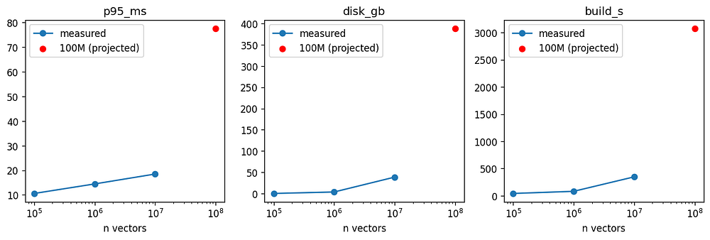
Measured p95 latency, disk, and build time across 100k to 10M, with the 100M projection in red (Created by
)
從 10 萬到 1000 萬所測得的 p95 延遲、磁碟與建置時間,一億的外推以紅色表示(由
製作)
At 100M vectors the projection lands at 77.58 ms p95 with a 388 GB index, which still fits on the NVMe disk of a single box. One caveat stated plainly.
在 一億個向量時,外推落在 77.58 毫秒的 p95、搭配一個 388 GB 的索引,這仍然放得進單一台機器的 NVMe 磁碟。有一個要坦白說明的告誡。
Recall at 10 sits near 0.1 here only because the vectors are random, which gives an approximate index almost nothing real to find, so this run measures latency and throughput, not retrieval quality. On a real corpus the same index keeps recall high, and the latency numbers are what hold as you scale.
這裡的 recall@10 之所以只落在 0.1 附近,純粹是因為這些向量是隨機的,這讓近似索引幾乎沒有任何真實的東西可找,所以這次執行衡量的是延遲與吞吐量(throughput),而非檢索品質。在一個真實的語料庫上,同樣的索引會維持高召回率,而那些延遲數字才是隨著你擴展時會維持不變的部分。
Where the time goes / 時間花在哪裡
Scale is the easy part. The expensive part is the per-query agent, so we attribute latency by stage to see where the budget actually goes.
規模是容易的部分。昂貴的部分是每次查詢的代理,所以我們按階段歸因(attribute)延遲,好看看預算實際上花到了哪裡。
def aggregate_latencies(results) -> "pd.DataFrame":
    stages = {}
    for r in results:
        for k, v in r.latencies.items():
            stages.setdefault(k, []).append(v)
    rows = [{"stage": k, "p50_s": round(np.percentile(v, 50), 3),
             "p95_s": round(np.percentile(v, 95), 3),
             "mean_s": round(np.mean(v), 3)} for k, v in stages.items()]
    return pd.DataFrame(rows).sort_values("mean_s", ascending=False)
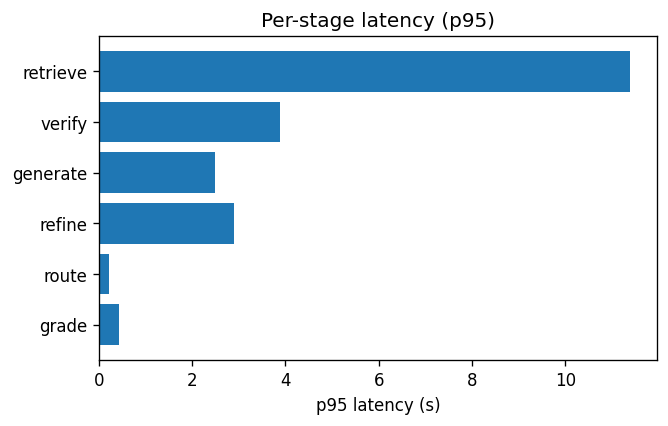
Per-stage p95 latency, where retrieval dominates the end-to-end budget (Created by
)
各階段的 p95 延遲,其中檢索主導了端到端(end-to-end)的預算(由
製作)
#### OUTPUT ####
   stage  p50_s  p95_s  mean_s
   total  4.001 17.668   5.823
retrieve  3.074 11.393   4.166
  verify  1.534  3.878   1.758
generate  1.451  2.484   1.619
  refine  1.471  2.888   1.575
   route  0.168  0.206   0.170
   grade  0.127  0.431   0.161
A typical question finishes in 4 seconds at the median, and the slow tail reaches 17.7 seconds at p95. Retrieve dominates, because it runs the embedder, both searches, and the cross-encoder reranker over 150 candidates, and on hard questions it runs more than once through the corrective loop.
一個典型的問題在中位數(median)約 4 秒完成,而緩慢的尾端在 p95 時來到 17.7 秒。檢索主導了一切,因為它要跑嵌入器、兩種搜尋、以及在 150 個候選上跑交叉編碼器重新排序器,而在困難的問題上,它會不只一次地跑過修正迴圈。
The vector search itself is the cheap part, which is the same lesson the scale lab taught. The index is not the bottleneck, the language model calls around it are.
向量搜尋本身才是便宜的部分,這和規模實驗室教會我們的教訓相同。索引不是瓶頸,環繞著它的那些語言模型呼叫才是。
That is worth knowing before optimizing, because it means the wins live in cutting model calls, batching the reranker, or caching grades, not in a faster vector store.
這在最佳化之前值得知道,因為它意味著勝利在於削減模型呼叫、把重新排序器批次化、或快取(cache)評分,而不在於一個更快的向量儲存。
Scope and What Comes Next / 適用範圍與接下來的方向
I want to close by being plain about what this is and what it is not. The hallucination rate is 2 percent on the unanswerable set, not zero, because literal zero is not achievable from a generative model.
我想在結尾坦白說明這是什麼、又不是什麼。幻覺率在不可回答集上是 2%,而不是零,因為從一個生成式模型身上,字面意義上的零是無法達成的。
Coverage on answerable questions is 0.46, which is the deliberate price we pay for that safety, and the risk-coverage curve is the dial for trading one against the other. The 10M run is a vector-search benchmark on synthetic vectors, so it proves the index scales in latency and disk, while a real corpus is what keeps recall high at the same speed.
可回答問題上的覆蓋率是 0.46,這是我們為那份安全刻意付出的代價,而風險-覆蓋率曲線就是拿一者去換另一者的那個旋鈕。那次一千萬的執行是一個在合成向量上的向量搜尋基準測試,所以它證明了索引在延遲與磁碟上能夠擴展,而一個真實的語料庫才是那個在相同速度下維持高召回率的關鍵。
The verifier sits at AUROC 0.702, which is good but not great, and it is the most valuable thing to improve next.
驗證器落在 AUROC 0.702,這不錯、但稱不上出色,而它是接下來最值得改進的東西。
From here, a few directions are worth the effort.
從這裡出發,有幾個方向值得投入心力。
- A stronger verifier: the gate is only as good as the judge, so a better faithfulness model lifts every downstream number at once.
-
一個更強的驗證器:關卡的好壞取決於評判者,所以一個更好的忠實度模型能一次提升每一個下游的數字。
-
Real embeddings at scale: rerun the scale lab over real document vectors to confirm recall holds while the 18 ms latency stays put.
-
規模下的真實嵌入:在真實的文件向量上重跑規模實驗室,以確認召回率維持不變、而 18 毫秒的延遲原地不動。
-
Sharding and quantization: past a single box, the index splits across shards, and the correctness logic above does not change at all.
-
分片(sharding)與量化:超出單一台機器之後,索引會拆分到各個分片上,而上面的正確性邏輯完全不會改變。
-
Calibrated coverage: tune the thresholds per domain so high-stakes corpora abstain more and casual ones answer more.
- 經過校準的覆蓋率:依領域調整門檻,好讓高風險(high-stakes)的語料庫多棄答一些、而隨性的語料庫多回答一些。
None of these next steps change the spine of the design. The index can grow, the verifier can improve, and the thresholds can move, but the contract stays the same. Every sentence that reaches a user is one the system could point to in the retrieved text, and everything else becomes an abstention.
這些接下來的步驟,沒有一個會改變這個設計的骨幹。索引可以成長、驗證器可以改進、門檻可以移動,但那份契約(contract)維持不變。每一句抵達使用者面前的話,都是系統能在檢索到的文字中指得出來的一句,而其餘的一切都變成一次棄答。
The whole thing is one idea carried all the way through. We do not try to make the model never wrong, we build a system that only ever says what it can prove, and abstains otherwise. The index scales to ten million vectors at 18 ms, the answers stay grounded at 0.908 faithfulness, and the questions it cannot support come back as a plain “I do not have enough evidence” instead of a confident guess.
整件事就是一個貫徹到底的理念。我們並不試圖讓模型永不出錯,我們建構的是一套只說它能證明的話、否則就棄答的系統。索引以 18 毫秒擴展到一千萬個向量,答案以 0.908 的忠實度維持有所依據,而它無法支持的問題會以一句樸素的「我沒有足夠的證據」回傳,而不是一個自信的猜測。
The full notebook, with every code cell and the real run outputs, is on GitHub:
完整的筆記本,連同每一個程式碼儲存格與真實的執行輸出,都在 GitHub 上:
[## GitHub - FareedKhan-dev/rag-zero-hallucinations: Handling 10M+ docs using RAG with zero…
Handling 10M+ docs using RAG with zero hallucinatons - GitHub - FareedKhan-dev/rag-zero-hallucinations: Handling 10M+…
github.com](https://github.com/FareedKhan-dev/rag-zero-hallucinations?source=post_page-----788e4b5b7f25---------------------------------------)
[## GitHub - FareedKhan-dev/rag-zero-hallucinations:使用 RAG 處理超過千萬份文件並達到零幻覺……
使用 RAG 處理超過千萬份文件並達到零幻覺 - GitHub - FareedKhan-dev/rag-zero-hallucinations:Handling 10M+……
github.com](https://github.com/FareedKhan-dev/rag-zero-hallucinations?source=post_page-----788e4b5b7f25---------------------------------------)
Wanna chat about RAG or anything else? Reach me on my LinkedIn.
想聊聊 RAG 或其他任何事情嗎?可以到我的 LinkedIn 找我。
🔤 關鍵術語
| 英文 | 繁中譯名 | 文章中的脈絡 / 簡短說明 |
|---|---|---|
| RAG (Retrieval-Augmented Generation) | 檢索增強生成 | 全文核心架構,透過檢索證據來約束生成、減少幻覺 |
| Hallucination | 幻覺 | 模型在缺乏證據時捏造內容;本文目標是「近乎零幻覺」 |
| Abstention | 拒答/棄權 | 當證據不足時系統選擇不回答,視為正確輸出而非失敗 |
| MinHash LSH | MinHash 局部敏感雜湊 | 以近似線性時間偵測近似重複段落,去除冗餘 |
| Structure-aware chunking | 結構感知分塊 | 依句子邊界打包至 token 預算,避免切斷實體語境 |
| Contextual retrieval | 情境化檢索 | 為每個 chunk 前綴一句情境說明,使其可獨立被檢索 |
| Hybrid index | 混合索引 | 同時儲存密集向量與稀疏 BM25,兼顧語意與精確詞 |
| Dense vector / embeddings | 密集向量/嵌入 | 捕捉語意改寫;以 Qwen3-Embedding 產生並正規化 |
| BM25 (sparse retrieval) | BM25(稀疏檢索) | 匹配專有名詞、ID、數字等精確 token |
| LanceDB | LanceDB | 內嵌式、可放於 NVMe 磁碟的向量庫,支撐 10M+ 向量 |
| Reciprocal Rank Fusion (RRF) | 倒數排名融合 | 僅依排名(非分數)融合密集與稀疏兩份排序清單 |
| Cross-encoder reranker | 交叉編碼器重排器 | 對 150 候選逐一評分,精排出前 20 名 |
| Query routing | 查詢路由 | 將問題分類為 no_retrieval / single_hop / multi_hop |
| Query decomposition | 查詢分解 | 將多跳問題拆成 2–3 個自足子問題再檢索 |
| Multi-hop question | 多跳問題 | 需結合多份文件事實才能回答的問題 |
| Cited generation | 帶引用生成 | 只依上下文作答,每句附段落 ID 引用,否則棄權 |
| Faithfulness judge / verifier | 忠實度評判器 | 以 32B LLM 檢查每條主張是否被引用文本支持 |
| Atomic claims | 原子主張 | 將答案拆成可獨立驗證的最小事實單位逐一查核 |
| Chain-of-Verification (CoVe) | 驗證鏈 | 對邊界答案重寫不受支持句子,再重跑驗證閘門 |
| CRAG loop | 校正式 RAG 迴圈 | 自我評分證據、弱則精修再檢索的自我校正 agent 迴圈 |
| IVF_PQ / ANN | IVF_PQ 近似最近鄰索引 | 分區+量化的近似檢索,10M 向量下 p95 僅 18 ms |
| AUROC | ROC 曲線下面積 | 在 HaluBench 上評估驗證器品質,得 0.702 |
| Risk-coverage curve | 風險—覆蓋率曲線 | 掃描門檻以在幻覺預算下最大化回答覆蓋率 |
| Context recall | 上下文召回率 | 檢索是否找回正確證據;本文達 0.97 |