Building Knowledge Graphs with Local LLMs: From Benchmarking to Fine-Tuning / 使用本地 LLM 建立知識圖譜:從基準測試到微調
Author: Alexander Shereshevsky
Published:
Source: https://medium.com/graph-praxis/building-knowledge-graphs-with-local-llms-from-benchmarking-to-fine-tuning-ed572268aa3f
Fetched: 2026-06-07T02:30:05.636204
Building Knowledge Graphs with Local LLMs: From Benchmarking to Fine-Tuning / 使用本地 LLM 建立知識圖譜:從基準測試到微調
Press enter or click to view image in full size
按 Enter 或點擊以檢視完整尺寸的圖片

For the production GraphRAG pipeline, the extraction step is where it quietly breaks.
對於正式環境的 GraphRAG 管線 (pipeline) 而言,抽取 (extraction) 步驟正是它悄悄出問題的地方。
I’ve been running a Graph RAG system for a while now. The idea behind it is compelling: instead of stuffing chunks of text into a vector store and hoping semantic similarity finds the right context, you build a knowledge graph — a structured network of entities and their relationships — and retrieve over that graph at query time. The system doesn’t just know what words appear near each other. It knows that Marie Curie worked at the University of Paris, that she discovered radium, and that radium is an element. That kind of structured understanding makes a real difference for complex questions that require connecting dots across multiple documents.
我已經運行一套 Graph RAG(圖譜檢索增強生成,Graph Retrieval-Augmented Generation)系統一段時間了。它背後的理念很有吸引力:與其把一段段文字塞進向量資料庫 (vector store),然後寄望語意相似度能找到正確的脈絡,不如建立一個知識圖譜 (Knowledge Graph)——一個由實體 (entity) 及其關係 (relationship) 構成的結構化網路——並在查詢時於該圖譜上進行檢索。這套系統不只知道哪些詞彙會出現在彼此附近,它知道居里夫人 (Marie Curie) 任職於巴黎大學、她發現了鐳 (radium),以及鐳是一種元素。對於需要跨多份文件串連線索的複雜問題,這種結構化的理解能帶來真正的差異。
But here’s what we don’t talk about enough: before you can query a knowledge graph, you have to build one.
但有件事我們談得還不夠:在你能夠查詢知識圖譜之前,你得先建立一個。
That means taking raw text — articles, legal filings, medical records, technical documentation — and extracting structured entity-relation triples from it. Things like (CRISPR-Cas9, developed_by, Jennifer Doudna) or (Tesla, headquartered_in, Austin). Most Graph RAG tutorials wave this away with a call to GPT-4. But we work with data that can't leave our infrastructure, which means we need local models. And local models have a much harder time with structured extraction than you might expect.
這意味著要拿原始文字——文章、法律文件、醫療紀錄、技術文件——並從中抽取出結構化的實體—關係三元組 (entity-relation triple)。像是 (CRISPR-Cas9, developed_by, Jennifer Doudna) 或 (Tesla, headquartered_in, Austin) 這樣的東西。大多數 Graph RAG 教學都用呼叫 GPT-4 一句帶過。但我們處理的資料不能離開我們的基礎設施,這意味著我們需要本地模型 (local model)。而本地模型在結構化抽取上的表現,比你想像中要困難得多。
We needed to understand exactly how hard this extraction problem is for our pipeline, and whether we could improve it. So we built a comprehensive internal benchmark, tested the leading open-weight models, and then fine-tuned one. This is what we learned.
我們需要確切了解這個抽取問題對我們的管線而言有多困難,以及我們能否改善它。於是我們建立了一套全面的內部基準測試 (benchmark),測試了領先的開放權重 (open-weight) 模型,然後微調 (fine-tune) 了其中一個。以下是我們學到的東西。
Part 1: The Benchmark / 第一部分:基準測試
What We Tested / 我們測試了什麼
We wanted to answer a practical question: if we hand a passage of text to a 7–9 billion parameter model running on our GPU infrastructure, how reliably can it extract a knowledge graph from it?
我們想回答一個實際的問題:如果我們把一段文字交給一個在我們 GPU 基礎設施上運行的 70 至 90 億參數 (parameter) 模型,它能多可靠地從中抽取出一個知識圖譜?
Internally, we built a large benchmark suite covering the domains our pipeline actually processes — hundreds of passages with hand-labeled gold-standard entities and triples across multiple complexity levels and document types. For this article, we’re sharing results from a representative 50-sample subset focused on the legal domain — contracts, case law, regulatory compliance, corporate governance, employment law, and international law — so that the findings are reproducible on public data. Each passage comes with gold-standard labels at four complexity levels: simple (a few clear entities), moderate (multiple interconnected relationships), complex (dense passages with nested relations), and edge cases (aliases, abbreviations, empty passages). This subset contains about 150 gold entities and 139 gold triples, and the patterns we observed here are consistent with those we see across the full internal benchmark.
在內部,我們建立了一套大型的基準測試套件,涵蓋我們管線實際處理的領域——數百段文字,附有跨多個複雜度層級與文件類型、人工標註的黃金標準 (gold-standard) 實體與三元組。在本文中,我們分享一個具代表性、聚焦於法律領域的 50 個樣本子集的結果——合約、判例法、法規遵循、公司治理、勞動法與國際法——好讓這些發現能在公開資料上重現。每段文字都附有四種複雜度層級的黃金標準標籤:簡單 (simple)(少數清楚的實體)、中等 (moderate)(多個相互關聯的關係)、複雜 (complex)(含巢狀關係的密集段落),以及邊緣案例 (edge cases)(別名、縮寫、空白段落)。這個子集包含約 150 個黃金實體與 139 個黃金三元組,而我們在此觀察到的模式,與我們在完整內部基準測試中看到的一致。
We tested four models, all running on a single NVIDIA RTX 3090 (24GB) via vLLM:
我們測試了四個模型,全部透過 vLLM 在單張 NVIDIA RTX 3090(24GB)上運行:
  Model                      Parameters   Family
 -------------------------- ------------ ----------------
  Qwen 2.5 7B Instruct       7B           Qwen (Alibaba)
  Llama 3.1 8B Instruct      8B           Llama (Meta)
  Mistral 7B Instruct v0.3   7B           Mistral
  Gemma 2 9B IT              9B           Gemma (Google)
Each model was tested with three prompting strategies: a naive instruction (“extract entities and relations as JSON”), a schema-in-prompt approach (same instruction plus the full JSON schema), and few-shot prompting (two worked examples showing the expected input-output format).
每個模型都用三種提示策略 (prompting strategy) 進行測試:天真指令 (naive instruction)(「以 JSON 抽取實體與關係」)、提示內嵌結構描述 (schema-in-prompt) 的做法(相同指令加上完整的 JSON 結構描述),以及少樣本提示 (few-shot prompting)(兩個展示預期輸入—輸出格式的範例)。
How We Measured Quality / 我們如何衡量品質
Evaluating extraction quality turns out to be almost as hard as doing the extraction itself. A model that outputs was_born_in instead of born_in is semantically correct — those mean the same thing in a knowledge graph. Penalizing that difference would make every model look worse than it actually is.
評估抽取品質,結果幾乎跟抽取本身一樣困難。一個輸出 was_born_in 而非 born_in 的模型在語意上是正確的——在知識圖譜中這兩者意思相同。為這種差異扣分,會讓每個模型看起來都比實際更糟。
We built an evaluation pipeline with three layers of fuzzy matching. First, entity matching uses token-sort ratio with a threshold of 75, so “Jennifer Doudna” matches “Dr. Jennifer Doudna” and partial overlaps are tolerated. Second, predicate matching goes through a synonym canonicalization layer — about 75 groups of semantically equivalent relationship names like {born_in, was_born_in, birthplace, place_of_birth} that all map to the same meaning. Third, substring matching handles cases in which a model produces verbose entity names within triples.
我們建立了一套具有三層模糊比對 (fuzzy matching) 的評估管線。首先,實體比對使用以 75 為閾值 (threshold) 的詞元排序比率 (token-sort ratio),因此「Jennifer Doudna」會匹配「Dr. Jennifer Doudna」,且容許部分重疊。其次,謂語 (predicate) 比對會經過一層同義詞正規化 (synonym canonicalization)——約 75 組語意等價的關係名稱,例如 {born_in, was_born_in, birthplace, place_of_birth},全都對應到相同的意義。第三,子字串 (substring) 比對處理模型在三元組中產出冗長實體名稱的情況。
These matching improvements increased the measured Triple F1 by 15–34% without altering any model outputs. The lesson: if you’re building a Graph RAG evaluation pipeline, invest as much in your matching logic as in your extraction prompts.
這些比對上的改進,在不改變任何模型輸出的情況下,將所測得的三元組 F1 分數 (Triple F1) 提升了 15 至 34%。這個教訓是:如果你正在建立一套 Graph RAG 評估管線,請在你的比對邏輯上投入和抽取提示同樣多的心力。
What We Found / 我們的發現
Entity detection is mostly solved. Relation extraction is not. All four models achieve Entity F1 between 0.78 and 0.91 — they’re quite good at finding things in text. But Triple F1 tells a different story. The best result across all 12 model-strategy combinations was 0.732 (Llama 3.1 with few-shot), and most configurations land between 0.52 and 0.60. Models can spot “Marie Curie” and “Warsaw” in a sentence, but reliably producing the structured triple (Marie Curie, born_in, Warsaw) is significantly harder.
實體偵測大致已被解決,關係抽取則否。 四個模型的實體 F1 (Entity F1) 都落在 0.78 到 0.91 之間——它們相當擅長在文字中找出東西。但三元組 F1 訴說的是另一個故事。在全部 12 種「模型—策略」組合中,最好的結果是 0.732(Llama 3.1 搭配少樣本),而大多數配置落在 0.52 到 0.60 之間。模型能在一個句子裡認出「Marie Curie」和「Warsaw」,但可靠地產出結構化三元組 (Marie Curie, born_in, Warsaw) 卻困難得多。
There’s no best model — there’s a tradeoff. This was the most practically important finding for our pipeline, and it held across the full internal benchmark. When we plotted schema conformance (does the model produce valid, parseable output?) against Triple F1 (when it works, how good is it?), the top-right corner was empty. No model was both highly reliable and highly accurate.
沒有最好的模型——只有取捨 (tradeoff)。 這是對我們的管線而言最具實際重要性的發現,而且它在整個內部基準測試中都成立。當我們把結構描述符合度 (schema conformance)(模型是否產出有效、可解析的輸出?)對三元組 F1(當它有效時,表現有多好?)作圖時,右上角是空的。沒有任何模型同時兼具高可靠性與高準確度。
  Model          Strategy           Schema Conformance   Triple F1
 -------------- ------------------ -------------------- -----------
  Llama 3.1 8B   few-shot           20%                  0.732
  Gemma 2 9B     few-shot           65%                  0.653
  Qwen 2.5 7B    few-shot           80%                  0.579
  Mistral 7B     few-shot           100%                 0.564
  Mistral 7B     schema-in-prompt   100%                 0.549
  Gemma 2 9B     schema-in-prompt   95%                  0.571
  Qwen 2.5 7B    schema-in-prompt   100%                 0.563
  Llama 3.1 8B   schema-in-prompt   95%                  0.522
Llama 3.1 with few-shot produces the best extractions when it works — but it only produces valid output 20% of the time. In a production pipeline, that means 80% of your documents either get dropped or need expensive retries. Mistral with schema-in-prompt never fails to produce valid JSON, but its extraction quality is mediocre. Gemma 2 sits in the middle, offering the best balance at 9B parameters.
Llama 3.1 搭配少樣本在有效時能產出最好的抽取結果——但它只有 20% 的時候會產出有效輸出。在正式環境的管線中,這意味著你 80% 的文件不是被丟棄,就是需要昂貴的重試 (retry)。Mistral 搭配提示內嵌結構描述從不會無法產出有效的 JSON,但它的抽取品質平庸。Gemma 2 居中,在 90 億參數的規模下提供了最佳的平衡。
Few-shot helps quality but hurts reliability. Across all four models, few-shot prompting consistently achieves the highest Triple F1. The worked examples help models understand the expected output structure and the granularity of predicates. But the cost is real: few-shot prompts are 3–5x longer, increasing latency and reducing output reliability. Longer contexts seem to confuse smaller models, leading them to produce malformed JSON or partial extractions. Mistral was the only model where few-shot was strictly better than the alternatives — it maintained 100% schema conformance even with the longer prompt.
少樣本有助於品質,卻有損可靠性。 在四個模型中,少樣本提示一致地達到最高的三元組 F1。這些範例幫助模型理解預期的輸出結構,以及謂語的粒度 (granularity)。但代價是真實存在的:少樣本提示長 3 到 5 倍,增加了延遲 (latency) 並降低了輸出可靠性。較長的脈絡似乎會讓較小的模型困惑,導致它們產出格式錯誤的 JSON 或不完整的抽取。Mistral 是唯一一個少樣本嚴格優於其他選項的模型——即使在較長的提示下,它仍維持 100% 的結構描述符合度。
Complexity degrades triples more than entities. When passages get harder — more entities, nested relationships, temporal qualifiers — entity detection stays relatively stable, but triple extraction drops sharply. The models struggle to decompose dense text into atomic triples, often producing compound objects instead of separate triples for each relationship. For our pipeline, which processes dense legal and technical text, this matters: extraction quality degrades more on our actual documents than simple benchmarks would suggest.
複雜度對三元組的劣化比對實體更嚴重。 當段落變得更困難時——更多實體、巢狀關係、時間限定詞 (temporal qualifier)——實體偵測維持相對穩定,但三元組抽取卻急劇下滑。模型難以將密集的文字分解成原子化的三元組 (atomic triple),常常產出複合的受詞 (compound object),而非為每個關係產出各自獨立的三元組。對於處理密集法律與技術文字的我們的管線而言,這很重要:抽取品質在我們的實際文件上的劣化,比簡單的基準測試所暗示的更嚴重。
Part 2: Closing the Gap with Fine-Tuning / 第二部分:以微調縮小差距
The benchmark results made the reliability-quality tradeoff painfully clear. In a production pipeline, you can’t tolerate 80% failure rates, but you also can’t accept mediocre extraction from models that happen to be structurally reliable. We needed to close this gap.
基準測試的結果讓可靠性與品質之間的取捨痛苦地清晰起來。在正式環境的管線中,你無法容忍 80% 的失敗率,但你也無法接受那些恰好在結構上可靠的模型所做出的平庸抽取。我們需要縮小這個差距。
The idea is straightforward. Instead of asking a general-purpose instruction-following model to perform structured extraction from a prompt alone, we teach it the pattern using supervised examples. After fine-tuning, the model should reliably produce valid JSON with entities and triples from a single short system prompt — no few-shot examples needed, freeing up the entire context window for longer passages.
這個想法很直接。與其要求一個通用的指令遵循 (instruction-following) 模型僅憑提示就執行結構化抽取,我們用監督式 (supervised) 範例來教它這個模式。微調之後,模型應該能僅憑一個簡短的系統提示 (system prompt) 就可靠地產出含有實體與三元組的有效 JSON——不需要少樣本範例,從而騰出整個脈絡視窗 (context window) 給更長的段落。
The Training Data / 訓練資料
For fine-tuning data, we turned to REBEL (Relation Extraction By End-to-end Language generation), a silver-labeled dataset from Babelscape built from Wikipedia text aligned with Wikidata triples. REBEL contains millions of text passages paired with their extracted entity-relation triples — exactly the task we need.
至於微調資料,我們轉向了 REBEL(透過端對端語言生成進行的關係抽取,Relation Extraction By End-to-end Language generation),這是一個由 Babelscape 製作、以銀標準 (silver-labeled) 標註的資料集,由維基百科文字與 Wikidata 三元組對齊建構而成。REBEL 包含數百萬段文字,並配對其抽取出的實體—關係三元組——正是我們需要的任務。
The raw REBEL format uses a linearized token scheme: <triplet> Subject <subj> Object <obj> Relation. We wrote a conversion pipeline that parses these into our target JSON format (entities with inferred types, plus subject-predicate-object triples), filters for quality (passages between 100-1500 characters, 2-15 triples each, deduplicated), and outputs chat-format JSONL ready for training.
原始的 REBEL 格式使用一種線性化的詞元方案 (linearized token scheme):<triplet> Subject <subj> Object <obj> Relation。我們寫了一套轉換管線,將這些解析成我們的目標 JSON 格式(帶有推斷型別的實體,加上主詞—謂語—受詞 (subject-predicate-object) 三元組)、依品質進行過濾(段落介於 100 至 1500 字元、每段 2 至 15 個三元組、去重),並輸出可供訓練的聊天格式 JSONL。
On top of that, we created 100 hand-crafted training samples spanning 30+ domains — physics, medicine, archaeology, computer science, ecology, telecommunications, and more — each with carefully labeled entities and triples. Blending high-quality curated examples with the larger silver dataset gives the model both precision and coverage.
在此之上,我們建立了 100 個人工精製的訓練樣本,橫跨 30 多個領域——物理學、醫學、考古學、電腦科學、生態學、電信等等——每個都附有仔細標註的實體與三元組。將高品質、精心整理的範例與較大型的銀標準資料集混合,能讓模型同時兼具精確度 (precision) 與涵蓋面 (coverage)。
The final training set: 3,000 samples from REBEL plus 100 hand-crafted samples, with 500 held out for validation.
最終的訓練集:來自 REBEL 的 3,000 個樣本加上 100 個人工製作的樣本,並保留 500 個作為驗證 (validation) 之用。
The Training Setup / 訓練設定
Press enter or click to view image in full size
按 Enter 或點擊以檢視完整尺寸的圖片
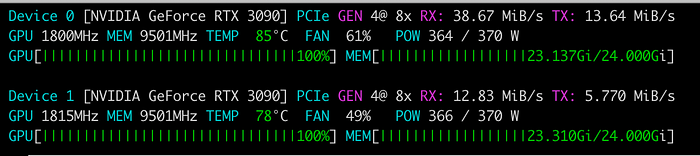
The training runs on two RTX 3090 GPUs using QLoRA — 4-bit quantized base weights with LoRA adapters on the attention and feed-forward projections. This keeps the memory footprint under 20GB per GPU while still enabling effective fine-tuning of an 8B-parameter model.
訓練在兩張 RTX 3090 GPU 上使用 QLoRA 運行——4 位元量化 (4-bit quantized) 的基礎權重,搭配置於注意力 (attention) 與前饋 (feed-forward) 投影上的 LoRA 適配器 (adapter)。這讓每張 GPU 的記憶體佔用維持在 20GB 以下,同時仍能對一個 80 億參數的模型進行有效的微調。
Key configuration choices, informed by the frontier training playbook:
以下是關鍵的配置選擇,參考了前沿訓練的最佳實務手冊 (playbook):
Base model: Qwen3–8B. It was among the top performers in our benchmark and uses the standard dense transformer architecture that fine-tunes predictably.
基礎模型:Qwen3–8B。 它是我們基準測試中表現頂尖者之一,並採用標準的密集 Transformer (dense transformer) 架構,微調行為可預測。
QLoRA with r=64, alpha=128. Higher rank than the typical r=16 default — structured extraction is a complex task and benefits from more adapter capacity. An alpha-to-rank ratio of 2 keeps the learning-rate scaling reasonable.
QLoRA 採用 r=64、alpha=128。 比典型的 r=16 預設值更高的秩 (rank)——結構化抽取是個複雜的任務,能受益於更多的適配器容量。alpha 對 rank 比值為 2,能讓學習率 (learning rate) 的縮放維持合理。
Learning rate: 3e-5 with cosine schedule. An order of magnitude below pretraining LR, following the playbook’s recommendation for SFT. Three epochs over the full dataset, with warmup over the first 3% of steps.
學習率:3e-5,搭配餘弦排程 (cosine schedule)。 比預訓練 (pretraining) 學習率低一個數量級,遵循該手冊對監督式微調 (SFT) 的建議。在完整資料集上跑三個訓練週期 (epoch),並在前 3% 的步數進行暖身 (warmup)。
User-turn masking. The training loss is computed only on the assistant’s output (the JSON extraction), not on the system prompt or the input passage. This focuses the model’s learning entirely on the extraction task.
使用者回合遮罩 (user-turn masking)。 訓練損失 (loss) 只在助理的輸出(即 JSON 抽取)上計算,而不在系統提示或輸入段落上計算。這讓模型的學習完全聚焦於抽取任務。
Sequence packing. Multiple short training examples are packed into a single sequence to maximize GPU utilization, since most extraction examples are well under the 2048-token limit.
序列打包 (sequence packing)。 多個簡短的訓練範例被打包進單一序列,以最大化 GPU 的利用率,因為大多數抽取範例都遠低於 2048 個詞元的上限。
The Results / 結果
Training completed in 33 minutes on 2x RTX 3090 GPUs. Final training loss: 1.0, validation loss: 0.67. The model converged smoothly — no training instability or loss spikes.
訓練在 2 張 RTX 3090 GPU 上於 33 分鐘內完成。最終訓練損失:1.0,驗證損失:0.67。模型平順地收斂 (converge)——沒有訓練不穩定或損失尖峰 (loss spike)。
We evaluated the fine-tuned model against the same 50-sample legal subset used for the base models. Here’s how the fine-tuned Qwen3–8B compares to the best base model configurations:
我們以與基礎模型相同的 50 個樣本法律子集來評估這個微調後的模型。以下是微調後的 Qwen3–8B 與最佳基礎模型配置的比較:
  Model                 Strategy                  Schema Conf.   Entity F1   Triple F1
 --------------------- ------------------------- -------------- ----------- -----------
  Qwen3-8B fine-tuned   finetune (naive prompt)   100%           0.847       0.211
  Llama 3.1 8B          few-shot                  20%            0.907       0.732
  Gemma 2 9B            few-shot                  65%            0.868       0.653
  Qwen 2.5 7B           schema-in-prompt          100%           0.814       0.563
  Mistral 7B            schema-in-prompt          100%           0.782       0.549
The results tell two very different stories depending on which metric you look at.
這些結果依你看哪個指標而訴說著兩個截然不同的故事。
The structural problem is completely solved. The fine-tuned model achieves 100% JSON validity and 100% schema conformance across all 50 samples. Every single response is a well-formed JSON object with the correct entity and triple structure. No parsing failures, no malformed output, no retries needed. For our pipeline, this is the single most important improvement — every parsing failure means lost data or expensive retry logic, and fine-tuning eliminates that entirely.
結構性的問題被徹底解決了。 微調後的模型在全部 50 個樣本上達到 100% 的 JSON 有效性與 100% 的結構描述符合度。每一個回應都是一個格式良好的 JSON 物件,具有正確的實體與三元組結構。沒有解析失敗、沒有格式錯誤的輸出、不需要重試。對我們的管線而言,這是單一最重要的改進——每一次解析失敗都意味著資料遺失或昂貴的重試邏輯,而微調徹底消除了這一點。
Entity extraction holds up well. At 0.847, Entity F1 is competitive with the base models — slightly below Llama’s 0.907 with few-shot but above Qwen 2.5’s 0.814 with schema-in-prompt. The model finds the right things in text.
實體抽取維持得很好。 實體 F1 為 0.847,與基礎模型相比具有競爭力——略低於 Llama 搭配少樣本的 0.907,但高於 Qwen 2.5 搭配提示內嵌結構描述的 0.814。這個模型能在文字中找出正確的東西。
But Triple F1 is disappointing — and the reason is illuminating.
但三元組 F1 令人失望——而其原因頗具啟發性。
The fine-tuned model scores 0.211 on Triple F1, well below every base model configuration. Looking at the raw outputs reveals exactly why. Here’s a sample extraction from the fine-tuned model on a legal passage about patent litigation:
微調後的模型在三元組 F1 上得到 0.211 分,遠低於每一個基礎模型配置。檢視原始輸出便能揭示確切的原因。以下是微調後模型針對一段關於專利訴訟的法律文字所做的抽取範例:
{
  "entities": [
    {"name": "TechCorp Industries", "type": "Organization"},
    {"name": "DataFlow Systems", "type": "Organization"},
    {"name": "U.S. Patent No. 10,234,567", "type": "Patent"}
  ],
  "triples": [
    {"subject": "TechCorp Industries",
     "predicate": "filed a patent infringement lawsuit against",
     "object": "DataFlow Systems"},
    {"subject": "TechCorp Industries",
     "predicate": "holds",
     "object": "U.S. Patent No. 10,234,567"}
  ]
}
The entities are correct. The triples are semantically correct — they accurately describe the relationships in the source text. But the predicate "filed a patent infringement lawsuit against" doesn't match the benchmark's gold predicate "filed_lawsuit_against". The model produces verbose, natural-language predicates instead of the concise snake_case identifiers the benchmark expects.
實體是正確的。三元組在語意上也是正確的——它們準確地描述了原始文字中的關係。但謂語 "filed a patent infringement lawsuit against" 與基準測試的黃金謂語 "filed_lawsuit_against" 不匹配。模型產出的是冗長的自然語言謂語,而非基準測試所預期的簡潔 snake_case 識別碼。
This is a domain transfer problem, not an extraction quality problem. The REBEL dataset — sourced from Wikipedia and Wikidata — uses encyclopedic, descriptive relation names. The model learned to extract relations in that style. Our legal benchmark uses terse, normalized predicates. The fuzzy evaluation pipeline’s 75 synonym groups help bridge some of this gap, but they can’t cover the full vocabulary mismatch between encyclopedic and domain-specific predicate styles.
這是一個領域遷移問題 (domain transfer problem),而非抽取品質問題。REBEL 資料集——來源為維基百科與 Wikidata——使用百科全書式、描述性的關係名稱。模型學會了以那種風格抽取關係。我們的法律基準測試使用的是簡潔、正規化的謂語。模糊評估管線的 75 組同義詞有助於彌合部分差距,但它們無法涵蓋百科式與領域特定謂語風格之間完整的詞彙不匹配。
But Wait — What About In-Domain Evaluation? / 但等等——領域內評估又如何呢?
The obvious next question: if the legal subset is unfair because of domain mismatch, what happens when we evaluate on held-out REBEL data — the same domain the model was trained on?
接下來顯而易見的問題是:如果法律子集因為領域不匹配而不公平,那麼當我們在保留的 REBEL 資料——也就是模型受訓的同一領域——上評估時,會發生什麼?
We ran exactly this experiment, generating 195 fresh REBEL samples (skipping the first 20,000 rows to avoid overlap with the training data) and evaluating the fine-tuned model on them.
我們正是做了這個實驗,產生了 195 個全新的 REBEL 樣本(跳過前 20,000 列以避免與訓練資料重疊),並在其上評估微調後的模型。
  Metric               Legal Subset   REBEL Held-Out
 -------------------- -------------- ----------------
  Samples              50             195
  JSON validity        100%           100%
  Schema conformance   100%           100%
  Entity F1            0.847          0.661
  Triple F1            0.211          0.067
Triple F1 on REBEL held-out data is worse than on the legal benchmark — 0.067 vs 0.211. That was genuinely surprising. The model was trained on REBEL data. How can it perform worse on more of the same?
在保留的 REBEL 資料上的三元組 F1 比在法律基準測試上更糟——0.067 對 0.211。這真的令人意外。模型是用 REBEL 資料訓練的。它怎麼會在更多同類資料上表現得更差?
Looking at the raw outputs reveals something deeper than a vocabulary problem. Here’s sample 35, a passage about figure skating competitions in Oberstdorf, Germany:
檢視原始輸出揭示了比詞彙問題更深層的東西。以下是第 35 號樣本,一段關於德國上施道夫 (Oberstdorf) 花式滑冰賽事的文字:
The REBEL gold triples are (Deutsche Eislauf-Union, country, Germany) and (Oberstdorf, country, Germany) — Wikidata-style facts linking entities to their country attribute. The model instead produces (Deutsche Eislauf-Union, organizes, competition) and (competition, location, Oberstdorf) — a natural reading of what the sentence actually says.
REBEL 的黃金三元組是 (Deutsche Eislauf-Union, country, Germany) 與 (Oberstdorf, country, Germany)——這是將實體連結到其國家屬性的 Wikidata 風格事實。而模型則產出 (Deutsche Eislauf-Union, organizes, competition) 與 (competition, location, Oberstdorf)——這是對句子實際所言的自然解讀。
Both extractions are correct. But they’re extracting different facts from the same text.
兩種抽取都是正確的。但它們從同一段文字中抽取的是不同的事實。
REBEL’s silver labels are derived by aligning Wikidata triples with Wikipedia sentences. When a sentence mentions Germany and Deutsche Eislauf-Union, REBEL looks up Wikidata and finds (Deutsche Eislauf-Union, country, Germany) — a knowledge base fact that happens to be supported by the sentence, even though the sentence isn't really about that fact. The model, meanwhile, learned to extract what the text actually describes: who organizes what, and where.
REBEL 的銀標準標籤是透過將 Wikidata 三元組與維基百科句子對齊而衍生出來的。當一個句子提到德國與 Deutsche Eislauf-Union 時,REBEL 會查詢 Wikidata 並找到 (Deutsche Eislauf-Union, country, Germany)——這是一個恰好被該句子支持的知識庫 (knowledge base) 事實,即使這個句子並非真的在講那個事實。與此同時,模型學會了抽取文字實際描述的內容:誰組織了什麼、在哪裡。
This is the difference between knowledge base completion (what facts do we know about these entities?) and text-grounded relation extraction (what relationships does this passage express?). REBEL trains on the former; the model internalized the latter. For Graph RAG — where the whole point is to build a knowledge graph that reflects what your documents actually say — the model’s behavior is arguably more useful than REBEL’s gold labels.
這就是知識庫補全 (knowledge base completion)(關於這些實體我們知道哪些事實?)與文字立基的關係抽取 (text-grounded relation extraction)(這段文字表達了哪些關係?)之間的差異。REBEL 是在前者上訓練的;模型則內化了後者。對於 Graph RAG 而言——其整個重點就是建立一個反映你的文件實際所言的知識圖譜——模型的行為可說比 REBEL 的黃金標籤更有用。
What This Actually Means / 這實際上意味著什麼
The fine-tuning result is both a success and a deeper lesson than expected.
這個微調結果既是一項成功,也是一個比預期更深刻的教訓。
What worked: Teaching a model to reliably produce structured JSON output through supervised fine-tuning is extremely effective. 100% schema conformance from a simple system prompt — no few-shot examples, no schema-in-prompt — is a significant practical win. In our pipeline, this eliminates the retry logic and failure handling that added latency and complexity to every extraction step.
有效的部分: 透過監督式微調來教導模型可靠地產出結構化 JSON 輸出,是極為有效的。僅憑一個簡單的系統提示——不需要少樣本範例、不需要提示內嵌結構描述——就達到 100% 的結構描述符合度,這是一項重大的實務勝利。在我們的管線中,這消除了那些為每個抽取步驟增添延遲與複雜度的重試邏輯與失敗處理。
What we learned about evaluation: Neither benchmark fairly measures this model. The legal subset penalizes predicate-vocabulary mismatches. The REBEL benchmark penalizes the model for extracting text-grounded relationships instead of knowledge-base-style facts. This highlights a fundamental challenge in relation extraction evaluation: there is no single “correct” set of triples for a given passage. The right extraction depends on what you’re building the knowledge graph for.
我們對評估學到的事: 這兩個基準測試都無法公平地衡量這個模型。法律子集懲罰謂語詞彙不匹配。REBEL 基準測試則懲罰模型抽取文字立基的關係而非知識庫風格的事實。這凸顯了關係抽取評估中的一個根本挑戰:對於一段給定的文字,並不存在單一「正確」的三元組集合。正確的抽取取決於你建立知識圖譜的目的是什麼。
What we’re doing next: The path forward for our pipeline is domain-specific fine-tuning data. Even 50–100 examples with our target predicate vocabulary and extraction philosophy — showing the model exactly what relationships matter for our use case — blended with the general REBEL base should close the gap. The model already knows how to extract; it just needs to learn what to extract for our domain.
我們接下來要做的事: 我們管線的前進之路是領域特定的微調資料。即使只是 50 至 100 個帶有我們目標謂語詞彙與抽取理念的範例——向模型展示對我們的使用情境而言究竟哪些關係重要——再與通用的 REBEL 基底混合,就應該能縮小差距。模型已經知道如何抽取;它只需要學會為我們的領域抽取什麼。
Part 3: Practical Takeaways / 第三部分:實務要點
Whether you’re running a Graph RAG pipeline today or evaluating whether to build one, here’s what this work suggests.
無論你今天正在運行一套 Graph RAG 管線,或是在評估是否要建立一套,以下是這項工作所提出的建議。
Start with schema-in-prompt. Across every model we tested, providing the JSON schema in the prompt is the safest default. It offers the best reliability-to-quality ratio and incurs almost no cost in terms of prompt length. Save a few shots for cases where you’ve validated it actually helps with your specific model and domain.
從提示內嵌結構描述開始。 在我們測試過的每個模型中,在提示裡提供 JSON 結構描述都是最安全的預設做法。它提供了最佳的可靠性對品質比值,而且在提示長度方面幾乎不增加成本。把少樣本留給那些你已驗證它確實對你的特定模型與領域有幫助的情況。
Budget for extraction failures. Even the most reliable base model configurations (Mistral + schema-in-prompt at 100% conformance) sacrifice extraction quality for reliability. Build your pipeline to handle failures gracefully — retry with a different strategy, fall back to a simpler extraction, or flag for human review.
為抽取失敗預留餘裕。 即使是最可靠的基礎模型配置(Mistral + 提示內嵌結構描述,達到 100% 符合度),也是以抽取品質換取可靠性。請把你的管線建造成能優雅地處理失敗——以不同策略重試、退回到較簡單的抽取,或標記交由人工審查。
Invest in evaluation. Overly strict string matching will make your models look 15–30% worse than they actually are. Build synonym-aware predicate matching and fuzzy entity comparison into your evaluation from day one.
投資於評估。 過於嚴格的字串比對會讓你的模型看起來比實際差 15 至 30%。從第一天起就把能感知同義詞的謂語比對與模糊實體比較納入你的評估之中。
Fine-tuning solves the reliability problem completely. If your pipeline suffers from parsing failures and malformed output, fine-tuning on a few thousand examples can eliminate these entirely. QLoRA on consumer GPUs, training in under an hour — the cost is minimal compared to the engineering time spent on retry logic and failure handling.
微調能徹底解決可靠性問題。 如果你的管線飽受解析失敗與格式錯誤輸出之苦,在數千個範例上進行微調就能徹底消除這些問題。在消費級 GPU 上用 QLoRA、在一小時內完成訓練——相較於花在重試邏輯與失敗處理上的工程時間,這個成本微不足道。
But mind the domain gap — it’s deeper than vocabulary. Fine-tuning on general-purpose extraction data like REBEL teaches the model the structural pattern, but it may learn a different extraction philosophy than you need. REBEL’s Wikidata-aligned labels favor knowledge-base completion; a production Graph RAG pipeline likely needs text-grounded extraction. Even a small set of domain-specific examples (50–100 samples) that show the model exactly which relationships matter for your use case will likely close this gap.
但要留意領域差距——它比詞彙更深層。 在像 REBEL 這樣的通用抽取資料上微調,會教給模型結構模式,但它可能學到與你所需不同的抽取理念。REBEL 對齊 Wikidata 的標籤偏好知識庫補全;而一套正式環境的 Graph RAG 管線很可能需要文字立基的抽取。即使是一小組領域特定的範例(50 至 100 個樣本),向模型展示對你的使用情境而言究竟哪些關係重要,也很可能彌合這個差距。
Evaluation is harder than extraction. Our REBEL experiment revealed that there’s no single “correct” set of triples for a given passage. A model that produces different but equally valid triples will score zero on any benchmark that expects specific gold labels. If you’re evaluating extraction quality, consider human evaluation of precision (are the extracted triples actually stated in the text?) alongside automated recall metrics.
評估比抽取更困難。 我們的 REBEL 實驗揭示了,對於一段給定的文字,並不存在單一「正確」的三元組集合。一個產出不同但同樣有效三元組的模型,在任何預期特定黃金標籤的基準測試上都會得到零分。如果你正在評估抽取品質,請考慮在自動化召回率 (recall) 指標之外,加入對精確度的人工評估(抽取出的三元組是否真的在文字中被陳述?)。
Local models are already production-viable. A Triple F1 of 0.55–0.65 from base models means more than half of the knowledge graph triples that a local model produces are correct and grounded in the source text. With confidence-based filtering and periodic human review, that’s enough to run a production knowledge graph without sending your data to external APIs.
本地模型已經可用於正式環境。 基礎模型 0.55 至 0.65 的三元組 F1 意味著本地模型所產出的知識圖譜三元組中,有超過一半是正確且立基於原始文字的。搭配基於信心度 (confidence) 的過濾與定期的人工審查,這已足以運行一個正式環境的知識圖譜,而無需將你的資料送往外部 API。
The gap between entity recognition and relation extraction is the real bottleneck in local Graph RAG. Closing it is a solvable engineering problem — not a fundamental limitation of the model size. The tools exist: open datasets like REBEL, efficient training with QLoRA, and a clear evaluation methodology to measure progress. The fine-tuning results show that structural reliability is already solved; the remaining challenge is teaching the model your domain’s extraction philosophy, which requires far less data than teaching extraction from scratch.
實體辨識 (entity recognition) 與關係抽取之間的差距,是本地 Graph RAG 真正的瓶頸。彌合它是一個可解決的工程問題——而非模型規模的根本限制。工具是現成的:像 REBEL 這樣的開放資料集、以 QLoRA 進行的高效訓練,以及一套用以衡量進展的清晰評估方法論。微調結果顯示,結構性的可靠性已經被解決;剩下的挑戰是教會模型你的領域的抽取理念,而這所需的資料遠少於從零開始教導抽取。
All experiments were run on NVIDIA RTX 3090 GPUs, using vLLM for inference and TRL/PEFT for fine-tuning. Sharing the adaptor training pipeline and REBEL conversion scripts on GitHub.
所有實驗均在 NVIDIA RTX 3090 GPU 上運行,使用 vLLM 進行推論 (inference),並使用 TRL/PEFT 進行微調。適配器訓練管線與 REBEL 轉換腳本分享於 GitHub。